6.3 Counting
We saw in Section 5.4 that the natural numbers correspond with the concepts of counting. These concepts form the foundation of finding probabilities of events, in particular compound events.
Related Content Standards
- (7.SPC.8) Find probabilities of compound events using organized lists, tables, tree diagrams, and simulation.
- Understand that, just as with simple events, the probability of a compound event is the fraction of outcomes in the sample space for which the compound event occurs.
- Represent sample spaces for compound events using methods such as organized lists, tables and tree diagrams. For an event described in everyday language (e.g., “rolling double sixes”), identify the outcomes in the sample space which compose the event.
Consider the following task:
Suppose that you are getting dressed and you have to choose a pair of jeans from three clean pairs and a shirt from your two clean shirts. How many different outfits could you have?
There are several different ways that one can work on this task. One method is to write down all of the possible combinations using an table. We see from this technique that we would have the following possible combinations:
| Shirt 1 | Shirt 2 | |
| Jeans 1 | Jeans 1 and Shirt 1 | Jeans 1 and Shirt 2 |
| Jeans 2 | Jeans 2 and Shirt 1 | Jeans 2 and Shirt 2 |
| Jeans 3 | Jeans 3 and Shirt 1 | Jeans 3 and Shirt 2 |
Another method of organizing the data is the use of tree diagrams
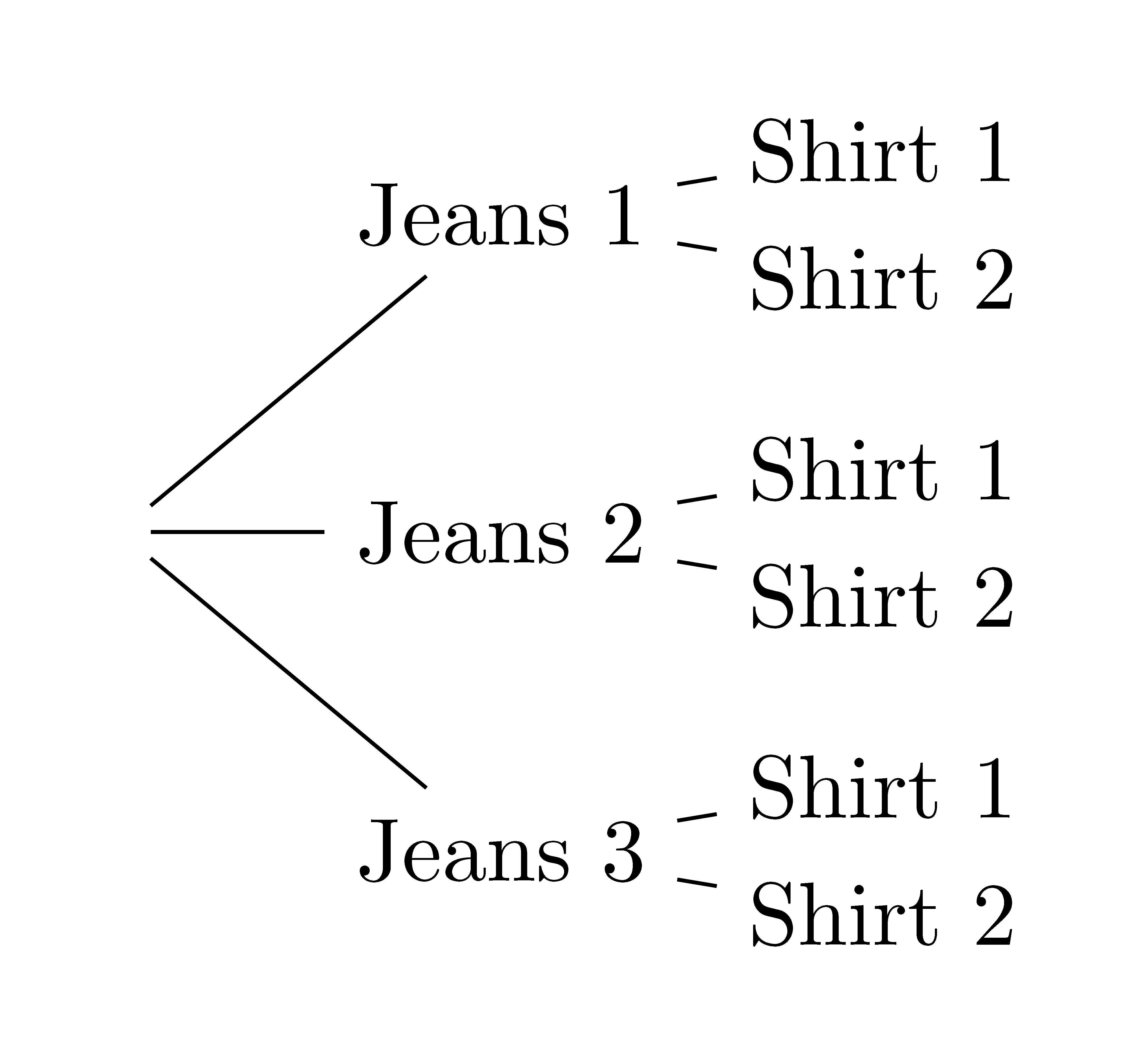
Both of these methods generate the same number of possible combinations are are extremely helpful for sets with a small number of elements. However, we can see that they would become very unwieldy with a large number of choices. So we would like to find a more compact and faster method. One pattern that we see from the table is that the number of options appears to follow the same structure as multiplication of the two numbers of choices, \(3\times 2 =6\). In order to prove this to be true, it is helpful to use the language of sets and cardinality.
6.3.1 Fundamental Counting Principle
Recall from Section 2.2.3 that \(A \times B= \{(a,b)\vert a\in A, b\in B\}\) is the set of ordered pairs of elements in \(A\) and \(B\) and is called \(A\) cross \(B\).
Theorem 6.4 (Multiplication Principle) Let \(A\) be a set with finite cardinality \(m\) and \(B\) be a set with finite cardinality \(n\). Then the set \(A\times B\) has cardinality \(mn\).
Proof. We will prove this theorem by fixing the natural number \(m\) and then using an induction argument for the second number, \(n\). So for each \(m,n\in \mathbb{N}\), we let \(P(m,n)\) be the statement: \[(\#(A) = m) \mbox{ and } (\#(B)=n) \Rightarrow \#(A \times B) = m \cdot n.\] Let \(m\in \mathbb{N}\) be fixed.
If \(n=0\), \(\#(B)=0\) and so \(B=\emptyset\) and so \(A\times B\) is also the empty set and has cardinality of \(0\). So \(P(m,0)\) is true.
If \(n=1\), \(\#(B)=1\) and so we can find a bijection from \(A\) to \(A\times B\) making \(\#(A\times B)=\#(A)\) and so \(P(m,1)\) is true.
We now assume that \(P(m,k)\) is true for some natural number \(k\). Let \(A\) be a set with cardinality \(m\) and \(B\) be a set with cardinality of \(k+1\). We can rewrite \(B\) as the union of two sets, one with cardinality of \(k\) that we will call \(B_k\) and one with cardinality of \(1\) that we will call \(B_1\). So \(B=B_k \cup B_1\), the disjoint union of the two sets. Using algebra of sets we can see that \[A\times B = A \times (B_k \cup B_1) = (A \times B_k) \cup (A \times B_1)\] and that \((A \times B_k) \cap (A \times B_1) = \emptyset\). Then Theorem 5.5, combined with the induction hypothesis, gives us that \[\# (A \times B) = \# (A \times B_k) + \# (A \times B_1) = (m\cdot k) + (m \cdot 1) = m\cdot (k+1).\] Therefore, \(P(m,k+1)\) is true, and by induction, \(P(m,n)\) is true for all natural numbers \(n\).
One can then extend this argument inductively to any finite number of finite sets. So, if we return to the clothing example, we let \(A\) be the set of options for Jeans (\(A=\{\mathrm{Jeans 1, Jeans 2, Jeans3}\}\)) and \(B\) the set of options for shirts (\(B=\{\mathrm{Shirt 1, Shirt 2}\}\)). Then \(\#(A)=3\), \(\#(B)=2\), and the number of possible outfits is \(3 \cdot 2 =6\). If we add an option of six different pairs of socks, the total number of possible outfits then increases to \(36\).
We can see that this technique is very useful in the process of determining the number of possible outcomes for compound events. Before we go into this further, we need to develop some additional mathematical language and terminology.
6.3.2 Factorial Notation
We saw in the previous section the usefulness of \(\binom{n}{k}\), and so we would like a quicker method for finding these values. In order to do so, we must first introduce factorial notation.
Definition 6.2 For \(n\in \mathbb{N}\) we define \(0!=1\) and for \(n>0\), \[n!=n\cdot (n-1) \cdot (n-2) \cdots (2)\cdot (1)\]
So we see that \(1!=1\), \(2!=2\cdot 1 = 2\), \(3!= 3 \cdot 2 \cdot 1 = 6\), \(4!= 4 \cdot 3 \cdot 2 \cdot 1 = 24\), and so on. We also see that \(n! = n \cdot (n-1)!\). This type of relationship lends itself well to induction arguments.
We can then use this factorial notation to write a compact formula for \(\binom{n}{k}\).
Theorem 6.5 For \(n,k\in \mathbb{N}\) with \(0\leq k \leq n\) we have that \[\binom{n}{k} = \frac{n!}{k!(n-k)!}.\]
Proof. As with many proofs of statements that involve the natural numbers, we will prove this using the principle of mathematical induction. For each pair of natural numbers \(n,k\) with \(0\leq k \leq n\) we let \(P(n,k)\) be the statement that \[\binom{n}{k} = \frac{n!}{k!(n-k)!}.\]
For \(n=0\), we know that \(k\) must equal \(0\), since that is the only number for which \(0\leq k \leq 0\). So to prove the \(P(0,0)\) is true we see that \[\frac{0!}{0!\cdot 0!} = \frac{1}{1} = 1\] and \(\binom{0}{0}=1\).
Then for \(n=m+1\) and \(k=0\), we see that \(\binom{n}{k} = \binom{m+1}{0} =1\) by the definition of Pascal’s triangle. And we see that \[\frac{(m+1)!}{0!(m+1-0)!}=1\] and so \(P(m+1,0)\) is true for all \(m\).
Similarly, for \(n=m+1\) and \(k=m+1\) \(\binom{n}{k}=\binom{m+1}{m+1}=1\), by definition of Pascal’s triangle. And we see that \[\frac{(m+1)!}{(m+1)!((m+1)-(m+1))!}=1\] and so \(P(m+1,m+1)\) is true for all \(m\).
We can now look at the induction step by assuming that for a natural number \(m>0\) the statement \(P(m,k)\) is true for all \(0\leq k \leq m\).
For \(n=m+1\) and \(0<k<m+1\) we see that \(\binom{n}{k}\) is defined using Pascal’s triangle by \[\binom{n}{k} = \binom{m+1}{k} = \binom{m}{k-1} + \binom{m}{k}.\] And by the induction hypothesis we see that \[\binom{n}{k} = \binom{m}{k-1} + \binom{m}{k} = \frac{m!}{(k-1)!(m-(k-1))!} +\frac{m!}{k!(m-k)!}\] and we can add the fractions using the common denominator of \(k!(m-k+1)!\). So \[\begin{align*} \binom{n}{k} &= \frac{k}{k}\frac{m!}{(k-1)!((m+1)-k)!} + \frac{m-k+1}{m-k+1} \frac{m!}{k!(m-k)!}\\ &= \frac{k(m!) + (m+1)(m!) -k (m!)}{k!((m+1)-k)!} \\ &= \frac{(m+1)!}{k!((m+1)-k)!} = \frac{n!}{k!(n-k)!} \end{align*}\] and so \(P(n,k)\) is true.
So by induction we see that \(P(n,k)\) is true for all natural numbers \(n,k\) with \(0\leq k \leq n\).
As we discussed in the previous section, Pascal’s triangle received its name because Pascal made connnections between this triangle of values and probability. We will now take some time to explore some of these connections by looking at permuations and combinations.
Related Content Standards
- (HSS.CP.8) Use permutations and combinations to compute probabilities of compound events and solve problems.
6.3.3 Permutations without Repetitions
A permutation of a set is a rearrangement of its elements into a linear order. So the permutations of the set \(\{1,2,3\}\) are often written as \[(1\: 2 \: 3), (1 \: 3 \: 2), (2 \: 1 \: 3), (2 \: 3 \: 1), (3 \: 1 \: 2), \mbox{ and } (3 \: 2 \: 1).\] One way that we can know how many of these permutations exist is to use some counting and organizing techniques. We can see that since we have three elements of the set, we have three options for the element put into the first position. Once the first element is chosen, we have two options for the second position. Once the first two positions are chosen, there is only one option for the third position. Because of this we can see that there are \(3\cdot 2 \cdot 1 = 3!\) different permutations of a set with three elements. We can continue this argument using inductive reasoning to see that there are \(n!\) different permutations of a set with \(n\) elements.
These types of permuations show up in the secondary curriculum with problems such as
In how many ways can 5 people arrange themselves in a row for a picture?
Sometimes a situation requires finding a permutation of \(n\) items into \(k\) positions, where \(k<n\).
If a class has 19 students, how many different arrangements can 4 students give a presentation to the class?
In these situations, we can use the multiplication principle to see that there are \[19\cdot 18 \cdot 17 \cdot 16 = 93,024\] different arrangements. This concept generalizes so that the number of \(n\) items into \(k\) positions is given by \(\frac{n!}{(n-k)!}\).
6.3.4 Permutations with Repetition
Sometimes we come across a situation in which the elements of the set can be chosen more than once.
A bike lock has a combination with 4 digits chosen from \(\{0,1,2,3,4,5,6,7,8,9\}\). How many different combinations exist?
We see using the Multiplication Principle that there are \(10\) choices for each of the \(4\) positions, \(10^4\). So if repetitions are allowed, the number of arrangements of \(n\) items into \(k\) positions is given by \(n^k\).
6.3.5 Combinations
For each of the permutations above, the order of the choices mattered. When this order does not matter, we call it a combination. For example, if we have a class of 21 students and we want to choose a group of 4 students to accomplish a certain task, then the order of the 4 students does not matter. And so we can find all of the possible permuations of the 21 students into 4 positions to get \(\frac{21!}{(21-4)!}\) different options. However, if we divide by the number of permutations of the 4 positions, \(4!\), then we would have the number of different groups, \[\frac{21!}{4!(21-4)!}.\]
We can generalize this into the following theorem.
Theorem 6.6 The number of ways an unordered set of \(k\) objects can be chosen from a set of \(n\) objects is given by \[\frac{\mbox{Number of ways to choose }k\mbox{ objects from } n \mbox{ in a specified order}}{\mbox{Number of ways the } k \mbox{ selected objects can be ordered}}\] \[ = \frac{\frac{n!}{(n-k)!}}{k!} = \frac{n!}{k!(n-k)!} = \binom{n}{k}\]
This theorem connects the counting technique of combinations with the binomial coefficients of Pascal’s triangle.
6.3.6 Summary
We combine all of these expressions into a single table for easy reference.
| Repeats Allowed | No Repeats | |
| Permutations (order matters) | \[n^k\] | \[\frac{n!}{(n-k)!}\] |
| Combinations (order doesn’t matter) | \[\frac{n!}{r!(n-k)!}\] |
One challenge in regards to Permutations and Combinations is to become too dependent on the formulas, rather than on the Principle of Multiplication underlying these concepts. For instance,
A State decides that they are issuing license plates for vehicles that have 7 symbols. The plate contains three letters and four numbers. In order to reduce confusion between the letter O and the number 0, they decide that neither of these symbols will be used. How many different license plates can the State create under these constraints?
This situation does not fit perfectly as either a Permutation or a Combination. Instead, it is a blend of the two.
6.3.7 Exercises
A coin is tossed 5 times.
- In how many ways is it possible to get two heads and three tails?
- In how many ways is it possible to get three heads and two tails?
- How are these two values related?
Discuss how the coefficients of the Binomial Theorem for \((x+y)^n\) relate to the number of ways of writing a product of \(k\) \(x\)’s and \((n-k)\) \(y\)’s.
How many distinguishable rearrangements of the letters of the word ‘Mississippi’ are there?
How many different ways can 5 people be arranged at a circular table so that two specific people are not sitting next to each other?