17.3 Hypothesis Testing
Following the order presented by Macdonald (1997) and Perezgonzalez (2015) we will introduce the historical development of two different views of hypothesis testing, with much of this material copied and adapted from Perezgonzalez (2015) under a Creative Commons license (CC BY).
17.3.1 Fisher’s Approach
Although some steps in Fisher’s approach may be worked out prior to the collect of data (e.g., the setting of hypotheses and levels of significance), the approach is eminently inferential and all steps can be set up once the research data is ready to be analyzed. Some of these steps can even be omitted in practice, as it is relatively easy for a reader to recreate them. Fisher’s approach to data testing can be summarized in the five steps described below. We will analyze data collected from the Census at School project to study the difference in the heights of thirteen-year-old students based on gender. The analysis will be conducted with random samples of 15 females and 15 males to simulate the type of data that might be collected in a classroom.
Step 1–Select an appropriate test.
This step calls for selecting a test appropriate to the research goal of interest, with a consideration of properties of the variable considered. A list of some of the basic tests and their uses is given below.
Correlational
Tests that look for an association between variables.
Pearson Correlation (\(\rho\)): Tests for the strength of association between two continuous variables (Definition 15.10)
Kendall’s Correlation (\(\tau\)): Tests for the strength of association between two ordinal variables (Definition 15.9)
Chi-Square (\(\chi^2\)): Tests for the strength of association between two categorical variables. (Not included in this text.)
Comparison of Means
Tests that look for the difference between the means of variables
Paired \(t\) or \(z\)-test: Tests for the difference between two variables from the same population (e.g. a pre- and post-test score). We use a \(t\) distribution for \(n<30\) and a \(z\) distribution for \(n\geq 30\).
Independent \(t\) or \(z\)-test: Tests for the difference between two variables from different populations (e.g. comparing two subgroups based on gender). We use a \(t\) distribution for \(n<30\) and a \(z\) distribution for \(n\geq 30\).
In our example comparing the heights of male and female thirteen-year-old students from the United States we will be using an independent \(z\)-test since the variable of height is continuous and the two samples are independent from each other.
Step 2–Set up the null hypothesis (\(H_0\)).
The null hypothesis (\(H_0\)) derives naturally from the test selected in the form of an exact statistical hypothesis (e.g., \(H_0: \mu_1-\mu_2 = 0\)). The states that in the population of interest there is no change, no difference, or no relationship regarding a certain property of a parameter. It is called the null hypothesis because it stands to be nullified with research data.
For the example of comparing heights for thirteen-year-old students we will set the null hypothesis to be that there is no difference in the heights of males and females, \[H_0: \mu_{\mbox{males}} - \mu_{\mbox{females}} = 0.\]
Directional and non-directional hypotheses. With some research projects, the direction of the results is expected (e.g., one group will perform better than the other). In these cases, a directional null hypothesis covering all remaining possible results can be set (e.g., \(H_0: \mu_1-\mu_2 \leq 0\)). With other projects, however, the direction of the results is not predictable or of no research interest. In these cases, a non-directional hypothesis is most suitable (e.g., \(H_0: \mu_1-\mu_2 = 0\)).
Step 3-Calculate the theoretical probability of the results under \(H_0\) (\(p\)).
Once the corresponding theoretical distribution is established, the probability (\(p\)-value) of any datum under the null hypothesis is also established.
When the sample size, \(n\), is small (generally less than 30) and the population standard deviation is unknown, we use a \(t\)-distribution as the theoretical distribution for the null hypothesis, usually with \(n-1\) degrees of freedom. For sample sizes larger than 30 we assume that the sample fits a normal distribution and we use the standard error as a substitute for the standard deviation of the population.
In our example of studying the heights of thirteen-year-old students, we find the male heights sample mean (173.47) and standard deviation (16.81) and female heights sample mean (164.73) and standard deviation (3.53). This produces a standard error for the difference of means of 4.43. Using this as the standard deviation of the distribution for the null hypothesis we can generate the following 1000 samples with mean of 0, based on a normal distribution.
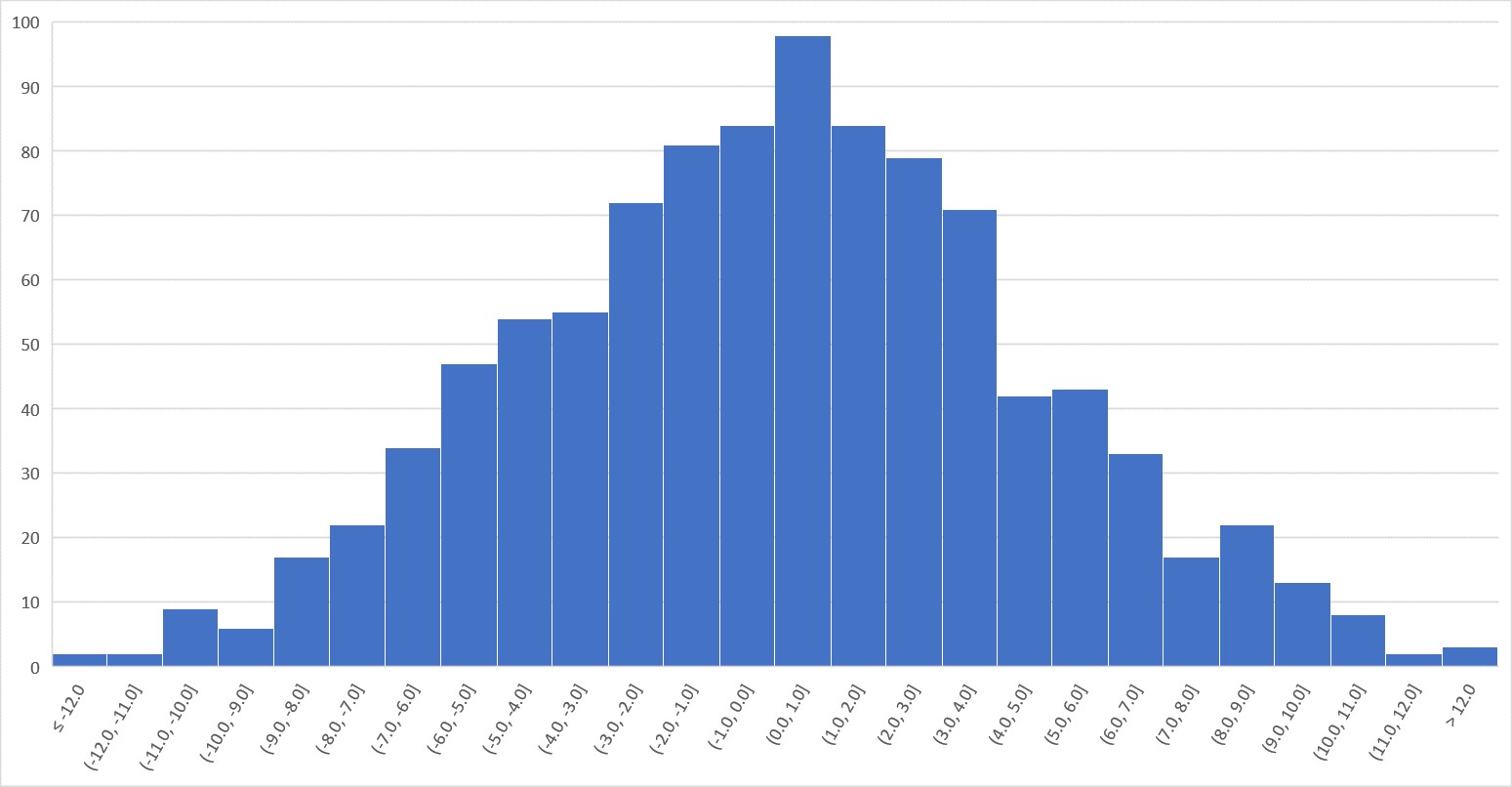
We see that data closer to the mean of the distribution, say between -5 and 5, have a greater probability of occurrence under the null distribution; that is, they appear more frequently and show a larger \(p\)-value (e.g., \(p = 0.72\), or 720 times in a 1000 trials). On the other hand, data located further away from the mean have a lower probability of occurrence under the null distribution.
The \(p\)-value comprises the probability of the observed results and also of any other more extreme results (e.g., the probability of the actual difference between groups and any other difference more extreme than that). Thus, the \(p\)-value is a cumulative probability rather than an exact point probability: It covers the probability area extending from the observed results toward the tail of the distribution. For our example a difference of 8.73 has a smaller \(p\)-value (e.g., \(p = 0.067\)). This means that if there is no difference between the heights of male and female thirteen-year-old students and the heights of these students follow a \(t\)-distribution with a mean of zero, if we generate 1000 samples of the same size as the one used, 67 of these samples would have a average difference in heights the same or larger than the one generated in our sample.
Step 4–Assess the statistical significance of the results.
Fisher proposed tests of significance as a tool for identifying research results of interest, defined as those with a low probability of occurring as mere random variation of a null hypothesis. A research result with a low \(p\)-value may, thus, be taken as evidence against the null (i.e., as evidence that it may not explain those results satisfactorily). How small a result ought to be in order to be considered statistically significant is largely dependent on the researcher in question, and may vary from research to research. The decision can also be left to the reader, so reporting exact \(p\)-values is very informative.
Overall, however, the assessment of research results is largely made bound to a given level of significance, by comparing whether the research \(p\)-value is smaller than such level of significance or not:
If the \(p\)-value is approximately equal to or smaller than the level of significance, the result is considered statistically significant.
If the \(p\)-value is larger than the level of significance, the result is considered statistically non-significant.
So if the \(p\)-value is less than the level of significance, we are more likely to reject the null hypothesis. Likewise, if the \(p\)-value is much larger than the level of significance we are less likely to reject the null hypothesis.
Level of significance. The level of significance is a theoretical \(p\)-value used as a point of reference to help identify statistically significant results. There is no need to set up a level of significance a priori nor for a particular level of significance to be used in all occasions, although levels of significance such as 5% or 1% may be used for convenience. This highlights an important property of Fisher’s levels of significance: They do not need to be rigid (e.g., \(p\)-values such as 0.049 and 0.051 have about the same statistical significance around a convenient level of significance of 5%).
Another property of tests of significance is that the observed \(p\)-value is taken as evidence against the null hypothesis, so that the smaller the \(p\)-value, the stronger the evidence it provides. This means that it is plausible to gradate the strength of such evidence with smaller levels of significance. For example, if using 5% as a convenient level for identifying results which are just significant, then 1% may be used as a convenient level for identifying highly significant results and 0.1% for identifying extremely significant results.
Step 5–Interpret the significance of the results.
Statistical Significance
A significant result is literally interpreted as a dual statement: Either a rare result that occurs only with probability \(p\) (or lower) just happened, or the null hypothesis does not explain the research results satisfactorily. Such literal interpretation is rarely encountered, however, and most common interpretations are in the line of “The null hypothesis did not seem to explain the research results well, thus we inferred that other processes—which we believe to be our experimental manipulation—exist that account for the results,” or “The research results were statistically significant, thus we inferred that the treatment used accounted for such difference.”
Non-significant results may be ignored, although they can still provide useful information, such as whether results were in the expected direction and about their magnitude. In fact, although always denying that the null hypothesis could ever be supported or established, Fisher conceded that non-significant results might be used for confirming or strengthening it.
In our case of comparing heights of male and female thirteen-year-old students, we found a difference in means of 8.73 cm with a \(p\)-value of 0.067. While this does not meet the standard threshold of 0.05, we can still argue that we should reject the null hypothesis that male students are the same height as female students. We may want to replicate this study with a new experiment with a larger sample size. By increasing the sample size, it is much more likely to obtain a difference that is statistically significant.
Practical Significance
Even if a result has statistical significance, it may not have practical significance. In our example of heights of thirteen-year-old students, we have to determine if a difference of around 9 cm matters within the context. This is often analyzed using percentages of the statistic being analyzed, i.e. 9 cm out of around 170 cm.
Highlights of Fisher’s approach
Flexibility.
Because most of the work is done a posteriori, Fisher’s approach is quite flexible, allowing for any number of tests to be carried out and, therefore, any number of null hypotheses to be tested (a correction of the level of significance may be appropriate).
Better suited for ad-hoc research projects.
Given above flexibility, Fisher’s approach is well suited for single, ad-hoc, research projects, as well as for exploratory research.
Inferential.
Fisher’s procedure is largely inferential, from the sample to the population of reference, albeit of limited reach, mainly restricted to populations that share parameters similar to those estimated from the sample.
No alternative hypothesis.
One of the main critiques to Fisher’s approach is the lack of an explicit alternative hypothesis, because there is no point in rejecting a null hypothesis without an alternative explanation being available. However, Fisher considered alternative hypotheses implicitly—these being the negation of the null hypotheses—so much so that for him the main task of the researcher—and a definition of a research project well done—was to systematically reject with enough evidence the corresponding null hypothesis.
17.3.2 Neyman and Pearson’s Approach
Jerzy Neyman and Egon Sharpe Pearson developed an alternative approach to data testing that is more mathematical than Fisher’s and does much of its work at the planning stage of the research project (Macdonald, 1997). It introduces a number of constructs, some of which are similar to those of Fisher and is summarized in the following eight main steps.
Step 1–Set up the expected effect size in the population.
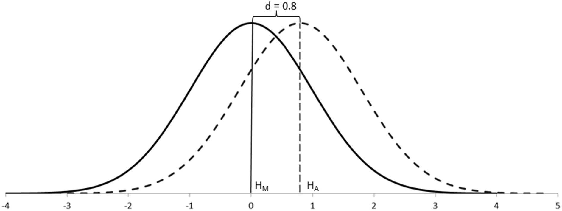
The main conceptual innovation of the Neyman-Pearson approach is the consideration of explicit alternative hypotheses when testing research data. In their simplest postulate, the alternative hypothesis represents a second population that sits alongside the population of the main hypothesis on the same continuum of values. These two groups differ by some degree: the .
For example, Cohen’s (1988) conventions for capturing differences between groups, \(d\), were based on the degree of visibility of such differences in the population: the smaller the effect size, the more difficult to appreciate such differences; the larger the effect size, the easier to appreciate such differences. Thus, effect sizes also double as a measure of importance in the real world.
When testing data about samples, however, statistics do not work with unknown population distributions but with distributions of samples, which have narrower standard errors. In these cases, the effect size can still be defined as above because the means of the populations remain unaffected, but the sampling distributions would appear separated rather than overlapping. Because we rarely know the parameters of populations, it is their equivalent effect size measures in the context of sampling distributions which are of interest.
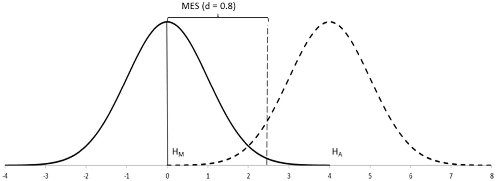
As we shall see below, the alternative hypothesis is the one that provides information about the effect size to be expected. However, because this hypothesis is not tested, the Neyman-Pearson approach largely ignores its distribution except for a small percentage of it, which is called \(\beta\). Therefore, it is easier to understand the approach if we peg the effect size to beta and call it the expected minimum effect size (\(\mbox{MES}\)). The minimum effect size effectively represents that part of the main hypothesis that is not going to be rejected by the test ( i.e., \(\mbox{MES}\) captures values of no research interest which you want to leave under the main hypothesis, \(H_M\)).
Step 2–Select an optimal test.
While the Neyman-Pearson approach allows for differentiation between tests described as the power of the test, the most common tests used are the same as those in the Fisher approach.
Step 3–Set up the main hypothesis (\(H_M\)).
The Neyman-Pearson approach considers, at least, two competing hypotheses, although it only tests data under one of them. The hypothesis which is the most important for the research (i.e., the one you do not want to reject too often) is the one tested. This hypothesis is better off written so as to incorporate the minimum expected effect size within its postulate (e.g., \(H_M: \mu_1-\mu_2 \in (0 - \mbox{MES}, 0 + \mbox{MES})\)), so that it is clear that values within such minimum threshold are considered reasonably probable under the main hypothesis, while values outside such minimum threshold are considered as more probable under the alternative hypothesis.
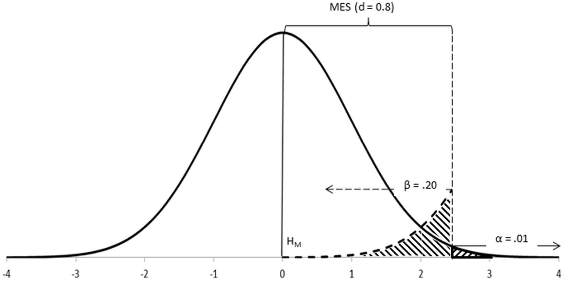
The main aspect to consider when setting the main hypothesis is the Type I error you want to control for during the research.
Definition 17.1 A Type I error (or error of the first class) is made every time the main hypothesis is wrongly rejected.
The alpha level, \(\alpha\), of a a hypothesis test is the probability that the test will lead to a Type I error.
Because the hypothesis under test is your main hypothesis, this is an error that you want to minimize as much as possible. Neyman and Pearson often worked with convenient alpha levels such as 5% (\(\alpha = 0.05\)) and 1% (\(\alpha= 0.01\)), although different levels can also be set. The main hypothesis can, thus, be written so as for incorporating the alpha level in its postulate (e.g., \(H_m: \mu_1-\mu_2 \in (0 - \mbox{MES}, 0 + \mbox{MES}), \alpha = 0.05\)), to be read as the probability level at which the main hypothesis will be rejected in favor of the alternative hypothesis.
Step 4–Set up the alternative hypothesis (\(H_A\)).
One of the main innovations of the Neyman-Pearson approach is the consideration of alternative hypotheses. The alternative hypothesis is written so as for incorporating the minimum effect size within its postulate (e.g., \(H_A: \mu_1-\mu_2 \notin (0 - \mbox{MES}, 0 + \mbox{MES})\)). This way it is clear that values beyond such minimum effect size are the ones considered of research importance.
Among things to consider when setting the alternative hypothesis are the expected effect size in the population (see above) and the Type II error you are prepared to commit.
Definition 17.2 A Type II error (or error of the second class) is made every time the main hypothesis is wrongly retained (thus, every time \(H_A\) is wrongly rejected).
Beta (\(\beta\)) is the probability of committing a Type II error in the long run and is, therefore, a parameter of the alternative hypothesis
Making a Type II error is usually less critical than making a Type I error, yet you still want to minimize the probability of making this error once you have decided which alpha level to use.
You want to make beta as small as possible, although not smaller than alpha (if \(\beta\) needed to be smaller than \(\alpha\), then \(H_A\) should be your main hypothesis, instead). Neyman and Pearson proposed 20% (\(\beta = 0.20\)) as an upper ceiling for beta, and the value of alpha (\(\beta = \alpha\)) as its lower floor. For symmetry with the main hypothesis, the alternative hypothesis can, thus, be written so as for incorporating the beta level in its postulate (e.g., \(H_A: \mu_1-\mu_2 \neq 0 \pm \mbox{MES}, \beta = 0.20\)).
Step 5–Calculate the sample size (\(N\)) required for good power (\(1-\beta\)).
Neyman-Pearson’s approach is predominantly dependent upon the process of designing the experiment or observation in order to ensure that the research to be done has good power. Power is the probability of correctly rejecting the main hypothesis in favor of the alternative hypothesis (i.e., of correctly accepting \(H_A\)). It is the mathematical opposite of the Type II error (thus, \(1-\beta\)). This means that we would want the power to be closer to 1 and the probability of a Type II error to be closer to 0.
| \(H_m\) True | \(H_m\) False | |
|---|---|---|
| Retain \(H_m\) | Decision Correct | Type II Error (probability \(\beta\)) |
| Reject \(H_m\) | Type I Error (probability \(\alpha\)) | Decision Correct (power \(1-\beta\)) |
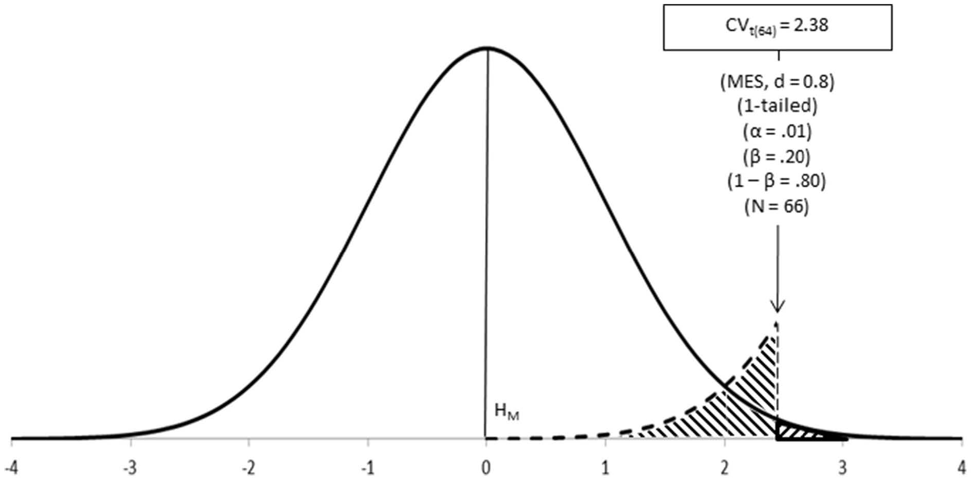
Step 6–Calculate the critical value of the test (\(\mbox{CV}_{\mbox{test}}\), or \(\mbox{Test}_{\mbox{crit}}\)).
Some of above parameters (\(\alpha\) and \(N\)) can be used for calculating the critical value of the test; that is, the value to be used as the cut-off point for deciding between hypotheses. We remember that as \(n\) increases, the probability of a Type I error (\(\alpha\)) and the probability of a Type II error (\(\beta\)) both decrease, while the power increases. So in the calculation of the critical value of the test, we are also determining the appropriate sample size in order to achieve our desired levels of \(\alpha\) and \(\beta\).
Step 8– Calculate the test value for the research.
In order to carry out the test, some unknown parameters of the populations are estimated from the sample (e.g., variance), while other parameters are deduced theoretically (e.g., the distribution of frequencies under a particular statistical distribution). The statistical distribution so established thus represents the random variability that is theoretically expected for a statistical main hypothesis given a particular research sample, and provides information about the values expected at different locations under such distribution.
Step 9 – Decide in favor of either the main or the alternative hypothesis.
Neyman-Pearson’s approach is rather mechanical once the design steps have been satisfied. Thus, the analysis is carried out as per the optimal test selected and the interpretation of results is informed by the mathematics of the test, following on the design set up for deciding between hypotheses:
- If the observed result falls within the critical region, reject the main hypothesis and accept the alternative hypothesis.
- If the observed result falls outside the critical region and the test has good power, accept the main hypothesis.
- If the observed result falls outside the critical region and the test has low power, conclude nothing.
17.3.2.1 Highlights of Neyman-Pearson’s Approach
More powerful.
Neyman-Pearson’s approach is more powerful than Fisher’s for testing data in the long run, as we can choose to accept or reject the two hypotheses. However, repeated sampling is rare in research.
Better suited for repeated sampling projects.
Because of above, Neyman-Pearson’s approach is well-suited for repeated sampling research using the same population and tests, such as industrial quality control or large scale diagnostic testing.
Less flexible than Fisher’s approach.
Because most of the work is done in the design stage, this approach is less flexible for accommodating tests not thought of beforehand and for doing exploratory research.
Defaults easily to Fisher’s approach.
As this approach looks superficially similar to Fisher’s, it is easy to confuse both and forget what makes Neyman-Pearson’s approach unique. If the information provided by the alternative hypothesis, \(\mbox{MES}\) and \(\beta\), is not taken into account for designing research with good power, data analysis defaults to Fisher’s test of significance.
17.3.3 Summary
In most research conducted, there is a blending of the two approaches. While this might make sense from a practical perspective, it does not maintain the same theoretical grounding of the original methodologies.
17.3.4 Exercises
A statistical analysis of a quantitative value of two groups of individuals is carried out and a test of the hypothesis that there is no difference between the two groups concerning that variable. The hypothesis test results in a \(p\)-value of \(0.01\). What would be an appropriate interpretation of this result?
The results of a hypothesis test are statistically significant for a significance level of \(\alpha=0.05\). What does this mean?