15.4 Measures of Center

Many of the graphical representations from the previous sections help to illuminate properties of the distribution of data along a single numerical variable. This section will provide ways to describe properties of such distributions numerically. These numerical descriptions provide additional ways to describe a distribution’s center, spread, and overall shape.

Related Content Standards

(6.SPA.2) Understand that a set of data collected to answer a statistical question has a distribution which can be described by its center, spread, and overall shape.
(6.SPA.3) Recognize that a measure of center for a numerical data set summarizes all of its values with a single number, while a measure of variation describes how its values vary with a single number.

One of the first attributes of a set of numerical data that most people want to know is a single number that describes the ‘average’ or ‘center’ of the data. Consider the following two questions:

What is the average height of students in 6th grade?
What is the height of the average student in 6th grade?

How are the questions similar and how are they different?

In addition to differences between wording, there are different ways to calculate the ‘average’. Consider the following three examples:

If a class of 25 students has 6 packages of cookies, with each package having 20 cookies, what is the average number of cookies that each person receives if the cookies are distributed evenly?
A motorboat makes a 24 mile upstream trip on a river against the current in 3 hours. The returning trip using the same amount of propeller rpm takes 2 hours. What is the motorboat’s average speed?
Your school was given a painting worth $5,000 4 years ago. The painting increased in value by 50% the first year, 20% the second year, and decreased by 10% the third year. It then increased by 5% this year. What is the average annual percentage increase over the 4 years?

With each of these three examples we are calculating a different type of average, or mean. Each of these means are equally based in mathematics and have usefulness in analyzing data.

In the first example of distributing cookies, we are computing the arithmetic mean that corresponds with even distribution of the quantity.

Definition 15.1 The arithmetic mean of values $a_1, a_2, \ldots a_n$ is defined by the formula: \[\mu = \frac{a_1 + a_2 + \cdots a_n}{n}.\]

The arithmetic mean is the most common center computed and is often called the average of the data. We see this particularly with spreadsheets where the function to compute the arithmetic mean is called Average.

In the cookie example we take the total number of cookies (120) and divide them evenly among the 25 students to have an average of 4.8 cookies per person.

Example 15.2 A group of 73 high school students participate in a walk-a-thon at their school⁷. The number of miles walked is represented in the following dot plot and has an arithmetic mean of 6.38 miles.

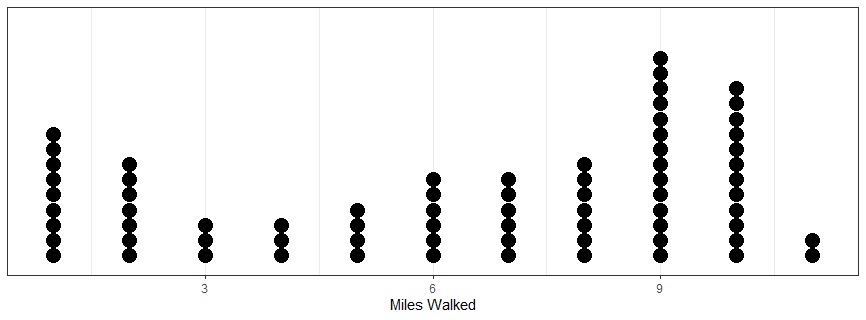
While we thought of the mean as an even distribution in the cookie example, in this example it is easier to think of the arithmetic mean as a balance point. If we think of the dot plot as a scale with each of the dots having the same weight, the scale is balanced at the point of 6.38.

When finding an average rate of change, one does not take the arithmetic mean of the values, but instead determines the total values of both quantities in the rate of change and then looks at the ratio. In the case of the motorboat, the total distance is 48 miles over a period of 5 hours, giving an average speed of 9.6 miles per hour.

This average of rates of change over equal intervals can be generalized using the harmonic mean.

Definition 15.2 The harmonic mean of values $a_1, a_2, \ldots a_n$ is defined by the formula: \[\frac{n}{\frac{1}{a_1} + \frac{1}{a_2} + \cdots + \frac{1}{a_n}}.\]

The harmonic mean is generally used to find the center of data that is a ratio of some type. Such situations include density (mass/volume) in physics, the price earnings ratio (price/earnings) in finance, and fuel economy (miles/gallon) for vehicles.

Example 15.3 When comparing different cities in the United States, it is sometimes useful to not just look at their overall populations, but to look at how many people there are per square mile. This gives a better impression of the density of the city, which usually corresponds to how big a city really feels.

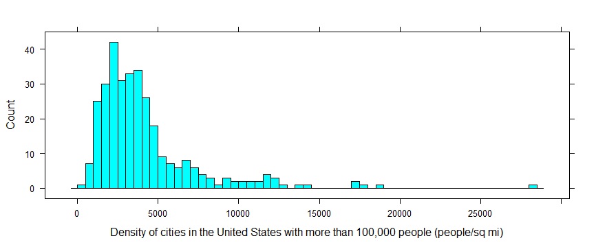
We see from the histogram above that New York City is an outlier in the data set. While the arithmetic mean is 4,171 people/sq mi, the harmonic mean is 2,641 people/sq mi. As we can see from the data, and the context of the variable, this harmonic mean is a better representation of the average density of these cities.

We now turn our attention to the example involving increases and decreases by a certain percentage. For this we are wanting to know what the equivalent percentage increase or decrease would be if it was constant over the four years. We see that the final amount of the painting can be found as \[1.05(0.90(1.20(1.50(5,000))))= \left( 1.05 \cdot 0.90 \cdot 1.20 \cdot 1.50\right) 5,000.\] So the equivalent amount of increase would be a $14\%$ increase, since $\sqrt[4]{\left( 1.05 \cdot 0.90 \cdot 1.20 \cdot 1.50\right)}=1.14$. This average of values is called the geometric mean.

Definition 15.3 The geometric mean of values $a_1, a_2, \ldots a_n$ is defined by the formula: \[\sqrt[n]{a_1 a_2 \cdots a_n}.\]

While the most common uses of the geometric mean involve compounded interest, the Water Quality Index produced by the EPA uses a geometric mean to combine multiple water quality indexes into a single index⁸. Using the geometric mean, rather than the arithmetic mean keeps individual extreme values on the sub-indexes from having a large effect on the overall index.

An additional common measure of the ‘center’ of a data set is the median.

Definition 15.4 The median is the value separating the higher half of a data sample, a population, or a probability distribution from the lower half.

The median of a sample is appropriate when the question about the data regards an ‘average case’, rather than an ‘average of cases’. We also generally use the median when the data set has extreme values on one end of the distribution, as these extreme values have a large effect on the arithmetic mean. For these reasons, variables such as salaries and home prices are usually best described with medians with the phrasing of ‘average salary’ or ‘average home price’.

Another time when a mean cannot be used, but a median can, is with ordinal variables. When there is not a set difference between consecutive values of a variable, the means of the variable do not have a good meaning. However, the median still makes sense. For instance, if we want to know how much education the average person in a sample has, we can sort the sample by the amount of education in number of years or type and then identify the educational level of the person in the middle of the distribution.

Example 15.4 There are some distributions for which the center is not a valuable piece of information. Consider the following graph of the starting salaries for lawyers in 2018⁹. The adjusted mean takes into account the expected under reporting of salaries by smaller companies.

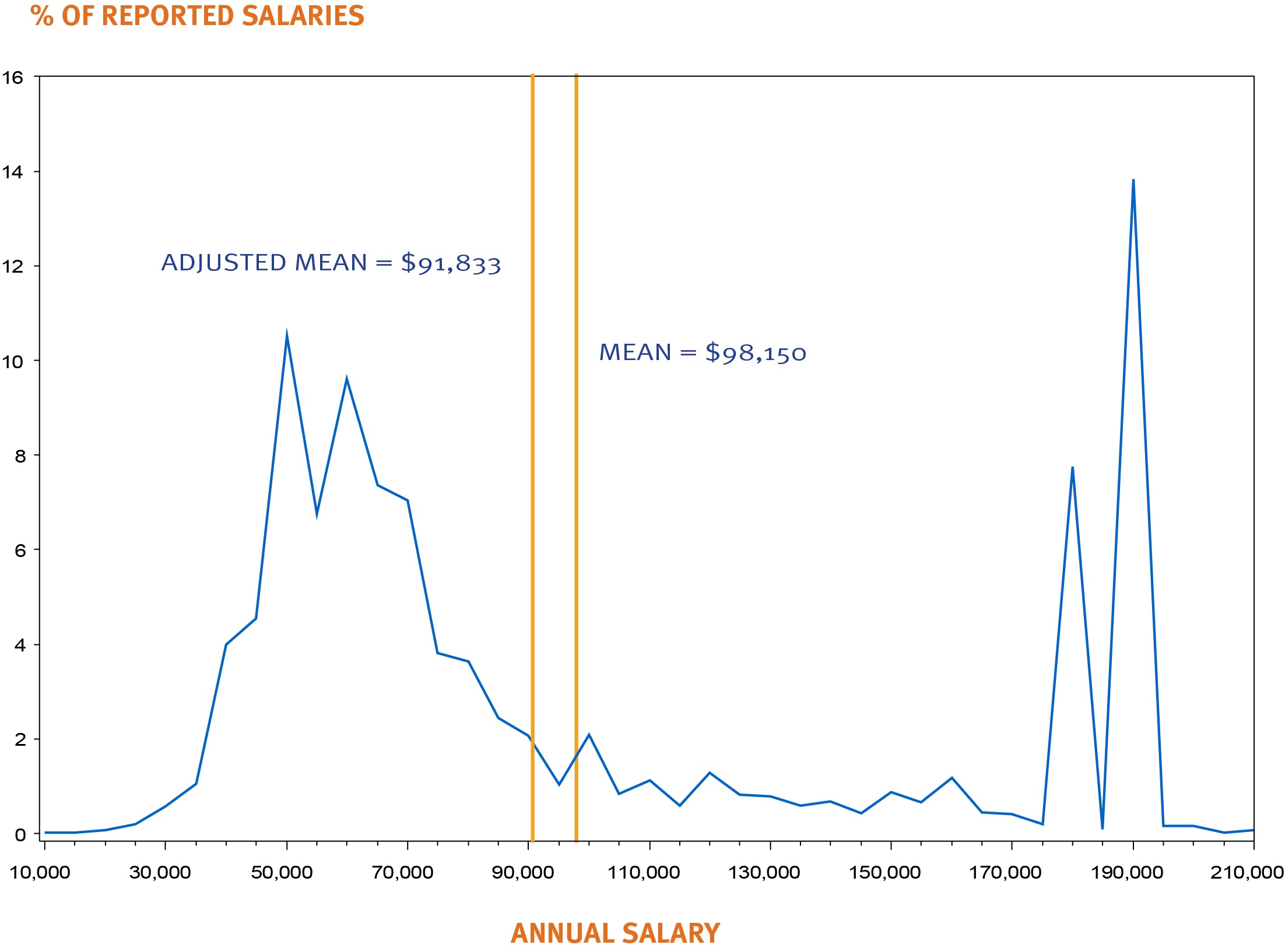
For this data set the adjusted mean of $91,833 is likely not much different from the median. However, there are not many lawyers fresh out of law school making that as their starting salaries. What are some other ways that the starting salaries of lawyers should be reported so that people can make a more informed decision about whether going to law school is a good choice for them?

Note: To help remember the difference between a mean and median, the mean is referred to as the ‘average of the data’, while the median is the ‘middle (average) entry in the data’.

15.4.1 Exercises

Is there a difference between the following two questions? (Justify your answer)
1. What is the average height of students in 6th grade?
2. What is the height of the average student in 6th grade?
3. How do the answers to these questions differ when accounting for gender?
Use Census at School data to provide answers to these questions for a sample of 500 6th grade students.
Download the current salaries of all players in the NFL.
1. What is the average salary of NFL players?
2. What is the salary of the average NFL player?
3. Why are these numbers similar or different? When would someone report one instead of the other?
4. How do these numbers compare to other professional sports?
Write a short paragraph explaining to your students how you would choose to use either the mean or the median.
Is there a relationship in terms of inequalities for any of the “averages” described in this section? (Test for relationships with 2 numbers in the data set.)