16.1 Probability Overview
Three main foundations of data analysis are trying to understand situations in their context, justification of claims using statistical techniques, and looking at the world through the lens of variability being everywhere. Probability is the study of uncertainty and is the foundation for understanding random variability. A phenomenon is considered to be random if there are multiple potential outcomes and there is uncertainty about which outcome will occur.
Phenomena like flipping a coin, drawing a ball from a bingo machine, or dealing a shuffled deck of cards are examples of physical randomness. We also have random selection in studies, which involves selecting a sample of individual cases at random from a population. Some examples are political polls to determine who people prefer in an election or biological samples from a stream to determine the overall health of the water source. Another use of randomness involves the random assignment of research participants into different control or experimental groups.
With random phenomena, there is uncertainty about individual outcomes, but there is a regular distribution of outcomes with a large enough number of repetitions. For instance, in the table below we give a few examples of simulated outcomes of coin flips for different numbers of repetitions.
| Number of Heads | Number of Tails | Proportion of Heads | |
|---|---|---|---|
| 3 Trials | 3 | 0 | 1.000 |
| 5 Trials | 3 | 2 | 0.6000 |
| 10 Trials | 4 | 6 | 0.4000 |
| 100 Trials | 52 | 48 | 0.5200 |
| 1,000 Trials | 492 | 508 | 0.4920 |
| 10,000 Trials | 4,995 | 5,005 | 0.4995 |
We can create such simulations using the RandBetween(0,1) function in a spreadsheet the appropriate number of times. Alternatively, we can use the mosaic package in R along with the commands coin <- c(0,1) and finding the mean of resamples by using mean(resample(coin,n)) where n is replaced by the number of trials.
This sampling technique demonstrates the phenomena that if someone could flip a fair coin an extremely large number of times that half of the time it would land on heads and half of the time it would land on tails. We can see here the use of simulations in studying various probability phenomena. One can do a simulation of a coin toss a thousand times in less than a minute using simulations, while conducting the experiment using a physical coin would take hours, or even days.
Just because something is a random phenomena does not mean that all of the outcomes have the same amount of certainty. For instance, in a Presidential election the tickets from the two major parties are much more likely to win the election than someone from a different party. Similarly, not all college football teams start the season with the same likelihood of winning a national championship.
Related Content Standards
- (7.SP.5) Understand that the probability of a chance event is a number between 0 and 1 that expresses the likelihood of the event occurring. Larger numbers indicate greater likelihood. A probability near 0 indicates an unlikely event, a probability around 1/2 indicates an event that is neither unlikely nor likely, and a probability near 1 indicates a likely event.
The probability of an event is a number in the interval \([0,1]\) measuring the likelihood of the event. We often describe these probabilities in terms of percentages with \(100\%\) corresponding to certainty and \(50\%\) corresponding to the event having the same likelihood of occurring or not occurring.
When there are only a finite number of possible outcomes we define the probability of a certain outcome as \[P(\mbox{certain event}) = \frac{\mbox{number of possible outcomes that correspond to the event}}{\mbox{number of all possible outcomes}}.\]
For instance, if we have a fair six-sided die the probability that we roll a number divisible by 3 is \(\frac{1}{3}\) because there are two number that are divisible by 3 out of the six possible numbers.
Since we know that there is a probability of \(\frac{1}{3}\) of rolling a number divisible by 3 on a fair six-sided die, we would expect that if we collected a large enough number of samples that about a third of the rolls would be a \(3\) or \(6\). As we increase the number of samples, we would expect the number of rolls to approach the theoretical probability.
Since the relative frequency of an event is the number of times that the event occurs during experimental trials divided by the total number of trials conducted, the predicted relative frequency of rolling a \(3\) or a \(6\) would be one third.
If we conducted an experiment where we roll a die a certain number of times, the long-run relative frequency of rolling a 3 or 6 should be around one third. The more times one rolls the die in the experiment, the more likely the long-run relative frequency will be closer to one third.
Consider the experiment of rolling a die 10, 50, and 100 times. The density plot below results from a simulation of 1000 cases of this experiment and we can see that the data is centered around \(\frac{1}{3}\).
In the case of 10 rolls, there is an point where none of the 10 rolls included a 3 or 6. We also can see that the standard deviation is \(1.146\). If we increase the number of rolls for each experiment up to 50 rolls, we see that more of the samples are within \(0.1\) of the expected probability of \(\frac{1}{3}\) and the standard deviation is reduced to \(0.067\). However, out of the 50 experiments there are some that substantially differ from the expected outcome. This demonstrates the randomness of the situation that all outcomes are still possible, even with a large number of trials.
As we continue to increase the number of rolls for each experiment up to 100 rolls, the variability in the distribution continues to decrease to the point that the standard deviation drops to \(0.046\). However, even with this decrease in standard deviation it is still possible to have experiments that differ greatly from the expected probability.
With the rolling of the dice, we can use the theoretical probability to predict the relative frequency and notice that increasing the number of trials greatly increased our accuracy. This phenomena of the average of the long-term relative frequency approaching the theoretical average as the number of cases increases is called the law of large numbers.
16.1.1 Compound Events
Most of the time that we calculate probabilities, the event space is more complicated and is a combination of multiple events. Such events are called compound events. We can use various techniques such as listing out all of the possible events and then work to determine the probabilities for each event, we can use tree diagrams to simplify the process of making sure that we have listed all of the possible events and computed their probabilities, or we can run simulations to estimate the probabilities of the combinations.
Related Content Standards
(7.SP.8) Find probabilities of compound events using organized lists, tables, tree diagrams, and simulation.
- Understand that, just as with simple events, the probability of a compound event is the fraction of outcomes in the sample space for which the compound event occurs.
- Represent sample spaces for compound events using methods such as organized lists, tables and tree diagrams. For an event described in everyday language, identify the outcomes in the sample space which compose the event.
- Design and use a simulation to generate frequencies for compound events.
Let’s assume that when a family has children, each child is equally likely to be a boy or girl. If a family has only one child, then we will denote the possible outcomes as \(B\) and \(G\) with both outcomes equally likely. If a family has two children, then we have four possible outcomes for the gender of the children in their birth orders, \(\{ BB, BG, GB, GG\}\). Each of these events are also equally likely. Another way to represent this information is through a tree diagram that lists all of the possible events and the probabilities of those events.
As we can see in the tree diagram, each of the four possible combinations has the same theoretical probability of occurring. However, in one example simulation of 200 families, we have the following probabilities: \[\mbox{BB: } 0.26 \quad \mbox{BG: } 0.20 \quad \mbox{GB: } 0.26 \quad \mbox{GG: } 0.28\]
In order to better understand the variability involved in family unit types, it is helpful to run simulations with large sample sizes. When we look at a sample of 50 simulations of 200 families, we have the following distribution for the proportion of the families with two boys. The sample had a mean of \(0.2511\) and standard deviation of \(0.0332\).
As we increase the size of our simulation and/or the number of simulations, we will find that the probabilities for each of the events in the simulation, \(0.2511\), will get closer to the theoretical probabilities found using the tree diagram, \(0.25\).
Related Content Standards
- (7.SP.7) Develop a probability model and use it to find probabilities of events. Compare probabilities from a model to observed frequencies; if the agreement is not good, explain possible sources of the discrepancy.
- Develop a uniform probability model by assigning equal probability to all outcomes, and use the model to determine probabilities of events.
- Develop a probability model (which may not be uniform) by observing frequencies in data generated from a chance process.
The tree diagram method of organizing the possible events and their probabilities is particularly useful when the probabilities are not all the same. In a deck of cards, there are 52 cards with 12 of them being face cards. Let’s explore the probabilities related to the number of face cards drawn in when drawing three cards. In the following tree diagram, we will denote the drawing of a face card by F and the drawing of a number card by N. Since we will be drawing cards and not replacing them, the probability of drawing face cards and number cards change as we draw the cards. For instance, if we draw a face card when we go to draw the next card there are a total of 51 cards to choose from and only 11 face cards left in the deck.
16.1.2 Estimating Probabilities
There are many times where we cannot determine the theoretical probability of an event, or doing so would be very difficult. In these cases, we frequently use a series of experiments or simulations to determine the long-run relative frequency of the event to approximate the probability of the event. In sports, we estimate a player’s probability of making a free throw, kicking a field goal, or hitting a home run by looking at the long-run relative frequency of those events in their past performances, either during the current game or throughout the season.
Related Content Standards
- (7.SP.6) Approximate the probability of a chance event by collecting data on the chance process that produces it and observing its long-run relative frequency, and predict the approximate relative frequency given the probability.
Example 16.1 Assume that a baseball player typically has four at-bats in a baseball game. If his hitting percentage is \(.253\), what is the probability of having at least three hits during the game?
We will see in a later section how to estimate this probability using theoretical probability techniques, but this can also be estimated using simulations.
Using the random number generator on a spreadsheet (=randbetween(1,1000)) one can designate a number less than or equal to 253 as a hit. We can do this four times to simulate a game of four at-bats. We can then create 500 of these possible games to estimate how many hits this player is likely to get.
| Number of hits in a game | 0 | 1 | 2 | 3 | 4 |
| Number of games with that many hits | 150 | 206 | 113 | 30 | 1 |
| Probability of that many hits | 30% | 41.2% | 22.6% | 6% | 0.2% |
So we see that the probability of having at least three hits during the game is estimated as \(0.06+0.002=0.062\), or \(6.2\%\).
The following “Birthday problem” was posed by Richard von Mises in 1939 (https://en.wikipedia.org/wiki/Birthday_problem):
How many people would need to be in a room so that it was more likely than not that at least two of them shared a birthday?
We can assume that all days of the year are equally likely to be a birthday and estimate this using a series of simulations by using a random number generator to generate a number between 1 and 365 to randomly generate a birthday. We can then choose different numbers of people in a room to estimate the probability of two people in the room sharing a birthday. Using simulations12 of 500 rooms we can estimate the probabilities of at least two people sharing a birthday for different numbers of people in the room.
| People in the room | 10 | 20 | 21 | 22 | 23 | 24 | 25 | 30 | 40 |
| Probability of a shared birthday | 13.8% | 37.4% | 46.2% | 49.8% | 53% | 53.8% | 60.8% | 70.4% | 88% |
We can see that if births were uniformly distributed throughout the year, we would need to have around 22 or 23 people in the room to have it more likely than not that two people share a birthday.
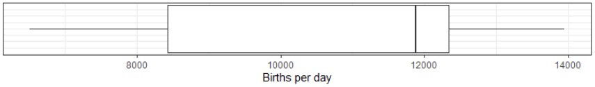
However, if we look at the number of people born in the United States in 201513 we see that there is a significant variability in the number of people born each day. So our assumption of a uniform distribution is not really met.
In order to work around the births not being uniformly distributed, we can use the birth data from 2015 to create 10,000 simulations using sampling into room populations from 20 to 30. We see that it still is around 22 people in a room to likely have two people share a birthday.
| People in the room | 21 | 22 | 23 | 24 | 25 |
| Probability of a shared birthday | 45.7 | 49.0% | 52.6% | 54.9% | 58.3% |
There are also times where events are not repeatable, but involve uncertainty; it is still reasonable to estimate the probability of the event. These include the probability of a certain team winning the national championship this year, or a certain candidate winning a presidential election. These are often referred to as subjective probability.
A common method to determine a subjective probability is the combination of observed data and statistical models to generate simulations that create a probability forecast of an event occurring. The probability of precipitation (or chance of rain) uses data collected from various weather stations to create models for the weather. These models are then analyzed with simulations to generate a probability that some minimum quantity of precipitation will occur within a specified forecast period and location.
The process of determining the probability of a team winning a national championship involves using predefined data, estimates of winning percentages for each game, and then running thousands of simulations of the entire season and reporting the percentage of those simulations that result in a championship.
16.1.3 Exercises
Gumballs14 - Imagine a gumball machine with 10 gumballs that always has 4 blue, 3 yellow, 2 green, and 1 red gumball. So, as you remove a gumball from the machine, it magically replaces it with the color you removed so that it always has the same proportion of colors.
- Create a physical (with marbles or cards) or computer simulation to answer the question, “If you took 10 gumballs out of the machine, how many of each color gumballs would you get?”
- How would the answer change if you had 50 people take out 10 gumballs?
- How would your answer change if 50 people took out 20 gumballs instead?
In the game of “Pass the Pigs” plastic pigs are rolled instead of dice. Since these are non-standard dice we do not know the probability of how each pig will land and so we need to run experiments to estimate the probability. Write up a plan for how you could have a class run experiments to estimate the probability for each of the possible ways for a pig to land.
In the example in this section about drawing face cards and number cards, we see that drawing three number cards is 400 times as likely to occur than drawing three face cards. How much more likely is it to draw a single face card of the three, than a single number card?
https://www.r-bloggers.com/the-birthday-paradox-puzzle-tidy-simulation-in-r/↩︎
Using the MosaicData package in R↩︎
Adapted from https://www.amstat.org/asa/files/pdfs/stew/TheGumballMachine.pdf↩︎