9.6 General Polynomial Functions
Now that we understand the graphs of quadratic polynomials we turn our attention to polynomials of higher degree. For all polynomials, the domain is the set of all real numbers. The range, however, are much harder to define and are much easier to determine using numerical methods in computer software.
9.6.1 Short-Term Behavior
Related Content Standards
- (HSA.APR.3) Identify zeros of polynomials when suitable factorizations are available, and use the zeros to construct a rough graph of the function defined by the polynomial.
We know that the graph of a polynomial \(p\) intercepts the horizontal axis at every point \(x=c\) such that \(p(c)=0\). We also know from the factor theorem that this corresponds to \(x-c\) being a factor of \(p(x)\). We say that \(p\) has a zero of order \(m\) at a point \(x=c\) if the prime factorization of \(p(x)\) includes \((x-c)^m\) as a factor, or equivalently \[p(x)=(x-c)^m \cdot q(x)\] where \(q(x)\) is a polynomial for which \(x-c\) is not a factor.
Theorem 9.1 Let \(p\) be a polynomial with a zero of order \(m\) at \(x=c\). Then \[p(x)=(x-c)^m \cdot q(x)\] where \(q(x)\) is a polynomial with \(q(c)\neq 0\). Furthermore, the Taylor polynomial of degree \(m\) for \(p\) centered at \(x=c\) is \[T_m(x)= q(c)\cdot (x-c)^m.\]
Before we prove this theorem, we will prove the following lemma.
Lemma 9.1 (General Leibniz Rule) Let \(f\) and \(g\) be \(n\)-times differentiable functions. Then \(fg\) is also \(n\)-times differentiable and \[(fg)^{(n)} (x) = \sum_{k=0}^n \binom{n}{k} f^{(n-k)}(x) g^{(k)}(x) \] where \[\binom{n}{k} = \frac{n!}{k!(n-k)!}.\]
Proof. Using a proof by induction argument we have the base case that \[(fg)'(x)=f'(x)g(x)+f(x)g'(x),\] which is the standard product rule for derivatives.
Now assume that the statement is true for some natural number \(j\). Then
\[\begin{align*} (fg)^{(j+1)}(x) &= \frac{d}{dx} \left( (fg)^{(j)}(x) \right) \\ &= \frac{d}{dx} \left( \sum_{k=0}^j \binom{j}{k} f^{(j-k)}(x) g^{(k)}(x) \right) \\ &= \left( \sum_{k=0}^j \binom{j}{k} \left( \frac{d}{dx} f^{(j-k)}(x) g^{(k)}(x) \right) \right) \\ &= \left( \sum_{k=0}^j \binom{j}{k} \left( f^{(j-k+1)}(x) g^{(k)}(x) + f^{(j-k)}(x) g^{(k+1)}(x) \right) \right) \\ &= \left( \sum_{k=0}^j \binom{j}{k} f^{(j-k+1)}(x) g^{(k)}(x) \right) + \left( \sum_{k=0}^j \binom{j}{k} f^{(j-k)}(x) g^{(k+1)}(x) \right) .\\ \end{align*}\] We can then re-index the second summation in order to have the order of the derivatives of \(f\) and \(g\) to align between the two summations, and we have that \[\begin{align*} (fg)^{(j+1)}(x) &= \left( \sum_{k=0}^j \binom{j}{k} f^{(j-k+1)}(x) g^{(k)}(x) \right) + \left( \sum_{k=1}^{j+1} \binom{j}{k-1} f^{(j+1-k)}(x) g^{(k)}(x) \right) \\ &= \binom{j}{0} f^{(j+1)}(x)g^{(0)}(x) + \left( \sum_{k=0}^j \left( \binom{j}{k} + \binom{j}{k-1} \right) f^{(j+1-k)}(x) g^{(k)}(x) \right) \\ & \quad \quad + \binom{j}{j} f^{(0)}(x)g^{(j+1)}(x) \\ \end{align*}\] Since \[ \binom{j}{0}= \binom{j+1}{0} = 1 \quad \mbox{and} \quad \binom{j}{j}= \binom{j+1}{j+1}=1\] and since
\[\begin{align*} \binom{j}{k} + \binom{j}{k-1} &= \frac{j!}{k! (j-k)!} + \frac{j!}{(k-1)!(j-(k-1))!} \\ &= \frac{j!\cdot (j-k+1)}{k! (j-k+1)!} + \frac{j! (k)}{k!(j-k+1)!}\\ &= \frac{j! (j+1)}{k! ((j+1)-k)!} = \frac{(j+1)!}{k! ((j+1)-k)!}\\ &= \binom{j+1}{k} \end{align*}\] we have that \[(fg)^{(j+1)}(x)= \sum_{k=0}^{j+1} \binom{j+1}{k} f^{((j+1)-k)}(x) g^{(k)}(x) \] and so the statement is true for \(j+1\).
Therefore, by induction we have that
\[(fg)^{(n)} (x) = \sum_{k=0}^n \binom{n}{k} f^{(n-k)}(x) g^{(k)}(x)\] is true for all \(n\).
Proof (Proof of Theorem 9.1). The factorization of \(p\) into \(p(x)=(x-c)^m \cdot q(x)\) is a direct consequence of Theorem 8.17.
Let \(f(x)=(x-c)^m\). Then multiple applications of the chain rule gives us that \[f^{(j)}(x) = \begin{cases} \frac{m!}{(m-j)!} (x-c)^{m-j} & \mbox{ if } 0 \leq j \leq m \\ 0 & \mbox{ if } j>m \end{cases}\]
Therefore, using the General Leibniz Rule we have that for \(0\leq n \leq m\), \[p^{(n)}(x) = \sum_{k=0}^n \binom{n}{k} \frac{m!}{(m-n+k)!} (x-c)^{m-n+k} q^{(k)}(x)\] and so \[p^{(n)}(c) = \begin{cases} 0 & \mbox{if } 0 \leq n < m\\ q(c) & \mbox{if } n=m \end{cases}\] giving us the result.
The key component of this theorem is that we can further understand how the graphs of polynomials behave near their zeros. If we let \[p(x)=x^6+x^5-11x^4-13x^3+26x^2+20x-24,\] we can write this in factored form and see that \[p(x)=(x-1)^2(x+2)^3(x-3)\] has a zero of order \(1\) at \(x=3\), a zero of order \(2\) at \(x=1\), and a zero of order \(3\) at \(x=-2\).
The theorem gives us a strong approximation of this polynomial near each of these zeros.
We have that near the zero at \(x=3\), \[p(x) \approx (3-1)^2(3+2)^3(x-3) = 500 (x-3).\]
Similarly, near \(x=1\), \[p(x) \approx -54 (x-1)^2.\]
Finally, near \(x=-2\), \[p(x)\approx -45 (x+2)^3.\]
By graphing these polynomials using computer software we can see that these approximations for the polynomial behavior near the zeros is much more accurate than the standard linear, quadratic, or cubic descriptions.
9.6.1.1 Complex Zeros
If \(p(x)\) is a polynomial in \(\mathbb{R}[x]\), the factors of this polynomial that correspond to complex zeros come in conjugate pairs. This means that if \((x-(a+bi))^j\) is a factor, then so is \(\overline{(x-(a+bi))^j}= (x-(a-bi))^j\).
While there is no direct correspondence between complex zeros and properties of the graph of a polynomial, if there are local minimum and maximum values for a polynomial for which the graph of the polynomial does not cross the horizontal axis, it implies that there are complex zeros of the polynomial.
9.6.2 Long-Term Behavior
When we study the long-term behavior of polynomials we focus on the standard form of the polynomial \[p(x)=a_0 + a_1 x + \cdots + a_n x^n \quad \mbox{ with } a_n\neq 0.\] When we look at the ratio of \(p(x)\) and its leading term \(a_n x^n\) we have \[\frac{p(x)}{a_n x^n} = \frac{a_0}{a_n} \frac{1}{x^n} + \frac{a_1}{a_n} \frac{1}{x^{n-1}} + \cdots \frac{a_{n-1}}{a_n} \frac{1}{x} + 1.\] So we see that \[\lim_{x \rightarrow \pm \infty} \frac{p(x)}{a_n x^n} =1\] meaning that these two functions act very similarly as \(|x|\) gets large.
This means that the graph of our polynomial \[p(x)=x^6+x^5-11x^4-13x^3+26x^2+20x-24\] will look very similar to the graph of its highest degree monomial, \(y=x^6\), when zoomed out to study its long-term behavior.
9.6.3 Polynomial Identities
Just like the difference of squares and perfect square for quadratic polynomials, there are some identities of polynomials that are very useful.
If \(p(x)=1+x+x^2+\cdots + x^{n-1}\) is multiplied by \((x-1)\) then one sees that \[\frac{x^n-1}{x-1} = 1+x+x^2+\cdots + x^{n-1}.\] This is the basis for the series \[\sum_{k=0}^\infty x^k = \frac{1}{1-x},\] along with understanding the roots of unity for complex numbers.
The identity \[(x^2+y^2)^2= x^4+2x^2y^2+y^4 = x^4-2x^2y^2+y^4+4x^2y^2 = (x^2-y^2)^2 + (2xy)^2\] can be used to generate Pythagorean triples. For instance, if \(x=2\) and \(y=1\) the identity becomes \(5^2=3^2+4^2\). If \(x=5\) and \(y=4\) we have the triple \(41^2=9^2+40^2\).
Finally, we have the identity
\[(x+y)^n = \sum_{k=0}^{n} \binom{n}{k} x^k y^{n-k}, \quad \mbox{ with } \binom{n}{k} = \frac{n!}{k!(n-k)!},\] which can be found using Pascal’s triangle (See 6.2).
Related Content Standards
- (HSA.APR.4) Prove polynomial identities and use them to describe numerical relationships.
- (HSA.APR.5) Know and apply the Binomial Theorem for the expansion of \((x + y)^n\) in powers of \(x\) and \(y\) for a positive integer \(n\), where \(x\) and \(y\) are any numbers, with coefficients determined for example by Pascal’s Triangle.
9.6.4 Exercises
For each of the following polynomials,
- What are the zeros of \(f\)?
- For what values of \(x\) is \(f(x)>0\)?
- For what values of \(x\) is \(f(x)<0\)?
- What is \({\displaystyle \lim_{x\rightarrow \infty} f(x)}\)?
- What is \({\displaystyle \lim_{x\rightarrow -\infty} f(x)}\)?
- \({\displaystyle f(x)=(3x+5)(x-1)(7x+3)(x-5)}\)
- \({\displaystyle f(x)=(2x-1)(3x+5)(x+1)}\)
- \({\displaystyle f(x)=(x-1)(4x+3)(3x-8)}\)
- \({\displaystyle f(x)=(2x+1)(3x-6)(x-6)}\)
For which values of \(k\) does the equation \[x^4-4x^2+x+k=0\] have four distinct real solutions?
If \(f(x)=3x^2\), what are all real values of \(a\) and \(b\) for which the graph of \(g(x)=ax^2+b\) is below the graph of \(f(x)\) for all values of \(x\)?
Consider the function \(f(x)=x^4-25x^2-36x\), which has one \(x\)-intercept at \((-4,0)\). Find all the other zeros of the function algebraically.
Determine the long-term behavior (Find \(\displaystyle{\lim_{x\rightarrow \infty} f(x)}\) and \(\displaystyle{\lim_{x\rightarrow -\infty} f(x)}\)) of the following polynomials.
- \({\displaystyle f(x)=2x^3-3x^2+4x-1}\)
- \({\displaystyle f(x)=-3x^4+2x^2-3x+2}\)
- \({\displaystyle f(x)=-5x^5+3x^4+2x^3-10x+15}\)
- \({\displaystyle f(x)=10x^6+7x^3-1}\)
For each of the zeros of the following polynomials, find the polynomial approximation of the same degree as the zero near the zero. (If \(f(x)\) has a zero of order \(m\) at \(x=c\), find the Taylor polynomial of degree \(m\) centered at \(x=c\), \(a_c (x-c)^m\).)
- \({\displaystyle f(x)=(x-1)(x+2)^2(2x-3)}\)
- \({\displaystyle f(x)=(2x+1)(x+3)^3(x-2)^2}\)
Assume the polynomial \(f\) has exactly two local maxima and one local minimum, and that these are the only critical points of \(f\).
- Sketch a possible graph of \(f\).
- What is the largest number of zeros \(f\) could have? (Explain your answer.)
- What is the least number of zeros \(f\) could have? (Explain your answer.)
- What is the least number of inflection points \(f\) could have?
- What is the smallest degree \(f\) could have?
- Find two possible formulas for \(f(x)\) with two different degrees.
Given the function \(f(x)=-x^4-3x^3+101x^2+543x+940\), use a graphing calculator to do the following:
- Find the zeros of the function. Round any zeros you find to the nearest tenth. Explain how you found your answer step-by-step, as if you were explaining to a student who does not know how to use a graphing calculator.
- Identify any local minima or maxima of the graph of the function as ordered pairs. Indicate which are local minima and which are local maxima. Round any minima or maxima to the nearest tenth. Explain how you found your answer step-by-step.
- Find the range of the function. Round the numbers in your answer to the nearest tenth. Explain how you found your answer step-by-step.
- Sketch the graph of the function. List a viewing window that shows all the information you found in the other parts of the problem. Explain why you chose your viewing window.
For each of the following graphs, give a possible algebraic representation for \(p(x)\).
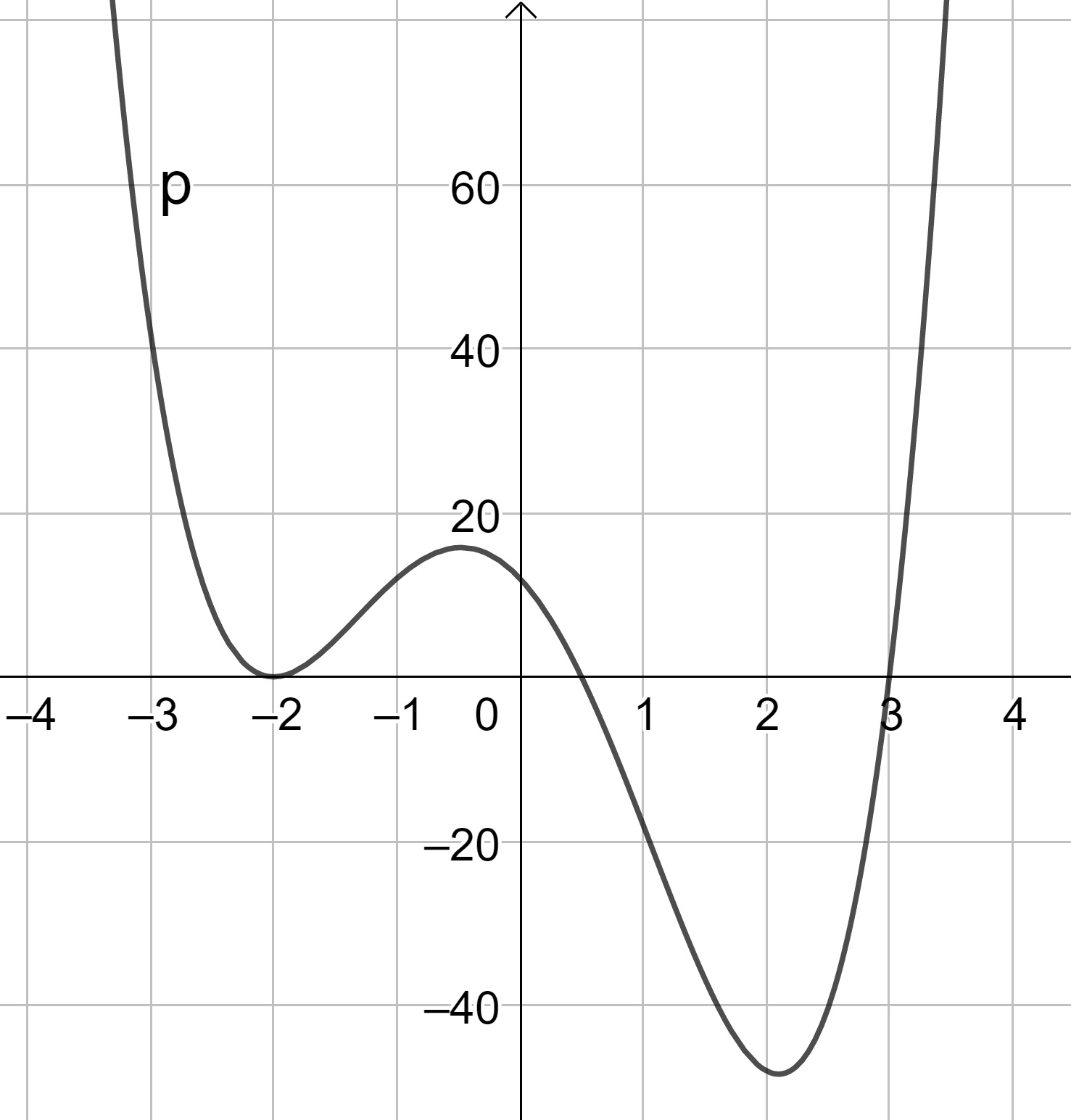
Figure 9.16: Graph 1
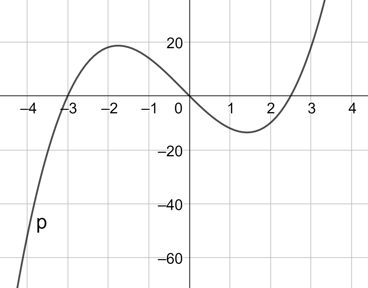
Figure 9.17: Graph 2
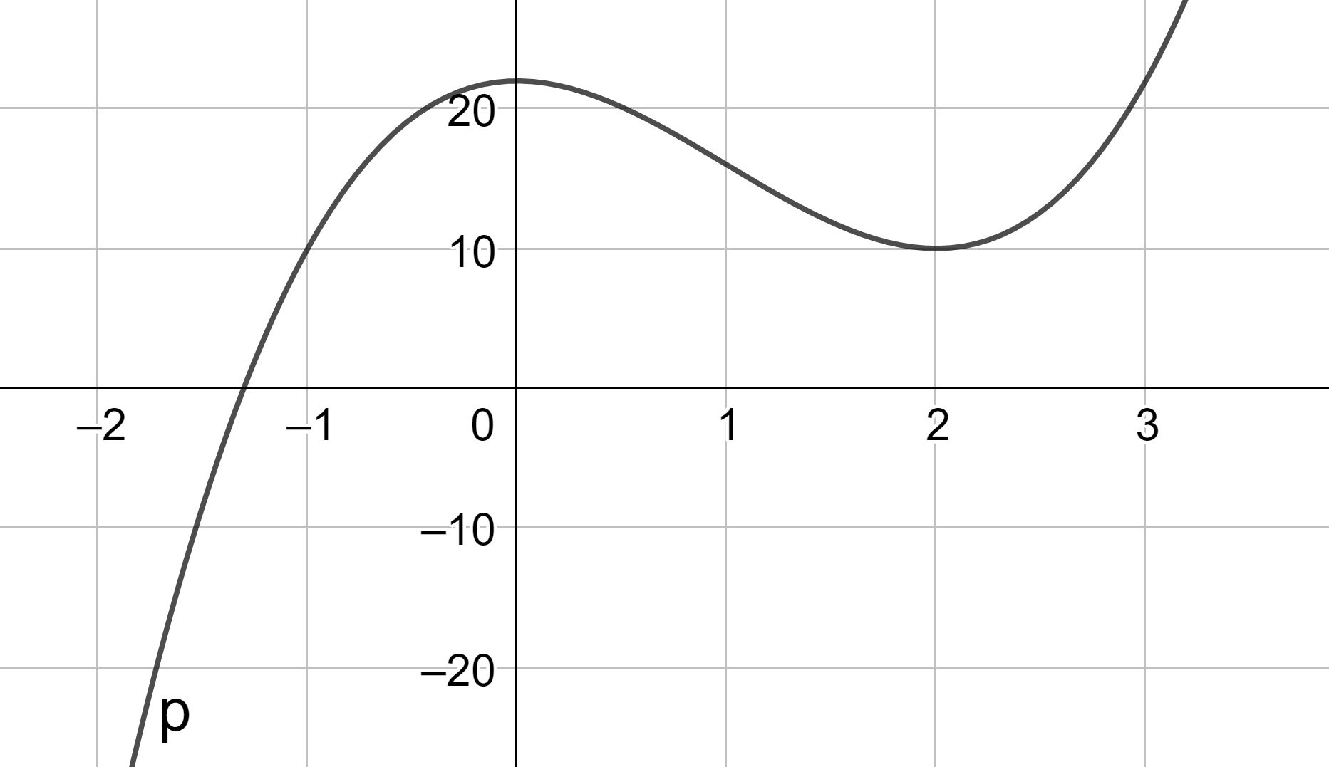
Figure 9.18: Graph 3