9.4 Linear Fractional Transformations

The function \(f(x)=\frac{1}{x}\) is another function that appears in physical applications such as Boyle’s law that the pressure of a given mass of an ideal gas is inversely proportional to its volume at a fixed temperature. In this section we will explore the family of functions that derive from this function. If \(f(x)=\frac{1}{x}\), then we see that for \(\alpha \neq 0\) and \(\beta \neq 0\) \[g(x)=\alpha \cdot f(\beta(x-h))+k = \frac{\alpha}{\beta} \cdot \frac{1}{ x- h} + k\] which can be rewritten as \[g(x)= \frac{\alpha + k(\beta x-\beta h)}{\beta x-\beta h}= \frac{(k\beta)x + (\alpha-\beta hk)}{\beta x-(\beta h)}= \frac{kx + \left(\frac{\alpha}{\beta} -hk\right)}{x-h}.\]

On the other hand, any function of the form \[h(x)=\frac{ax+b}{cx+d}\] can be rewritten in the form \[h(x)= \frac{a}{c} - \left( \frac{ad-bc}{c^2}\right) \frac{1}{x+\frac{d}{c}}\] and so we see that it is a transformation of the inverse proportional function if and only if \(ad-bc \neq 0\) and \(c\neq 0\).

If we allow \(c=0\), then the functions are transformations of both the linear and inversely proportional parent functions.

Therefore, the family of functions whose parent function is either \(f(x)=\frac{1}{x}\) or \(f(x)=x\) we call linear fractional transformations (also called a Möbius transformations) as a real-valued function of the form \[f(x)=\frac{ax+b}{cx+d}\] where \(a\), \(b\), \(c\), and \(d\) are real-valued constants with \((ad-bc)\neq 0\).

9.4.1 Domain

Let \[f(x)=\frac{ax+b}{cx+d}\] where \(a\), \(b\), \(c\), and \(d\) are real-valued constants with \((ad-bc)\neq 0\).

If \(c\neq 0\), then these functions are not defined at the point \(\frac{-d}{c}\) and so the natural domain for the function would be \(\mathbb{R}\setminus \left\{\frac{-d}{c}\right\}\).

If \(c=0\), then \(d\neq 0\) and so we see that the function becomes a linear function of the form \[f(x)= \frac{a}{d} x + \frac{b}{d},\] and so the domain of the function is \(\mathbb{R}\).

9.4.2 Range

If \(c\neq 0\), the parent function for these functions is inversely proportional function so that \[f(x)=\frac{ax+b}{cx+d} = \frac{a}{c} -\left(\frac{ad-bc}{c^2}\right)\frac{1}{x+\frac{d}{c}}\]

So for this case that \(c\neq 0\), we see that this function is a transformation of the parent function that takes transforms the plane so that the horizontal axis maps to the horizontal line of \(y=\frac{a}{c}\), and so the range of the function is \(\mathbb{R}\setminus \{\frac{a}{c}\}\).

If \(c=0\), the linear fractional transformation reduces to a linear function whose range is \(\mathbb{R}\).

9.4.3 Increasing or decreasing

Using the graph of \(y=\frac{1}{x}\) we can sketch a graph of the transformation of this function.

Figure 9.13: Transformations of \(f(x)=1/x\)

By using the expression of the linear fractional transformation of \[f(x)=\frac{ax+b}{cx+d}= \frac{a}{c} - \left(\frac{ad-bc}{c^2}\right) \frac{1}{x+\frac{d}{c}}\] we see that if \(ad-bc>0\) that \(f\) is increasing on \((-\infty, \frac{-d}{c})\) and on \((\frac{-d}{c}, \infty)\). We also see that if \(ad-bc<0\) that the function is decreasing on these intervals.

9.4.4 Intercepts

From the primary algebraic expression of the function, one can see that if \(a\neq 0\) the horizontal intercept of the function is at \(\frac{-b}{a}\), and if \(a=0\) that there is no horizontal intercept.

One can also see that if \(d \neq 0\) that the vertical intercept is at \(\frac{b}{d}\) with no vertical intercept if \(d=0\).

9.4.5 End behavior and asymptotes

One can see from the graph of \(f(x) = \frac{ax+b}{cx+d} = \frac{a}{c} - \left(\frac{ad-bc}{c^2}\right) \frac{1}{x+\frac{d}{c}}\) that \[\lim_{x\rightarrow \pm \infty} f(x) = \frac{a}{c}\] and that the behavior near the vertical asymptote of \(x=-\frac{d}{c}\) depends upon the sign of \(ad-bc\).

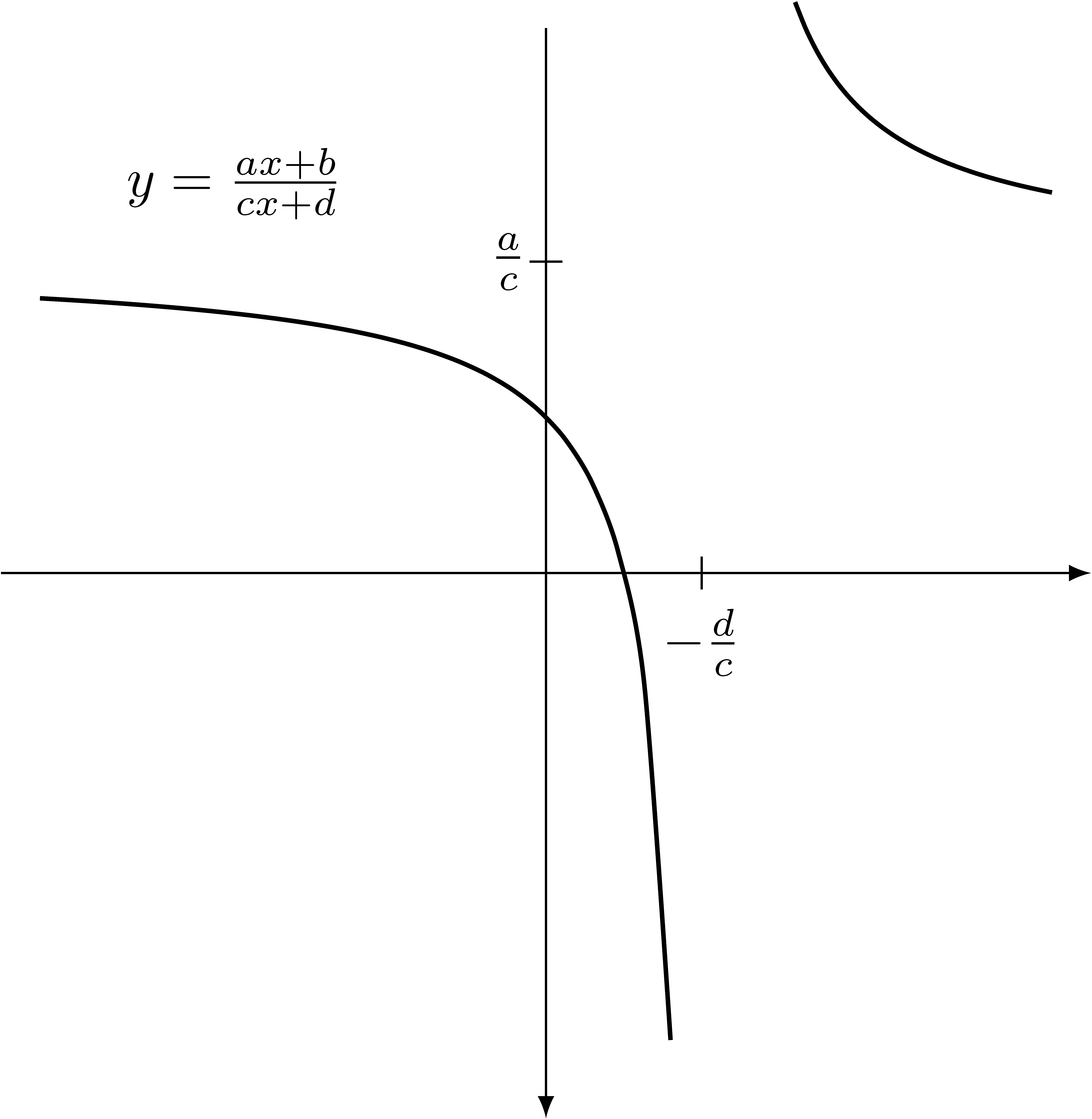
Figure 9.14: General Linear Fractional Transformation

9.4.6 Extensions

By adding a single element to the set of real numbers that we will call \(\infty\), we can redefine these functions to have both a domain and range of \(\mathbb{R}\cup \{\infty\}\). If \(c\neq 0\) we define \(f\) on this extended domain to be \[f(x)= \begin{cases} \frac{ax+b}{cx+d}, & x\in \mathbb{R} \setminus \{-\frac{d}{c}\} \\ \frac{a}{c}, & x = \infty \\ \infty , & x = -\frac{d}{c} \end{cases}\] and if \(c=0\), \[f(x)= \begin{cases} \frac{a}{d} x + \frac{b}{d}, & x \in \mathbb{R} \\ \infty , & x= \infty \end{cases}.\]

For the ease of notation, we will denote these extended functions by the algebraic representation of the original function and imply the extension to the extended real numbers.

From the results above about range and monotonicity of the function we can see that the linear fractional transformations on these extended domains and co-domains are bijections. That leads us to want to understand the forms of the inverse function and the composition of two of these linear fractional transformations.

In order to understand more about the composition of two linear fractional transformations we will define \[f(x)=\frac{ax+b}{cx+d} \mbox{ and } g(x)=\frac{\alpha x + \beta}{\gamma x + \delta}.\] Then we have that \[\begin{align*} (g\circ f) (x) & = \frac{\alpha \left(\frac{ax+b}{cx+d}\right) + \beta}{\gamma \left( \frac{ax+b}{cx+d}\right) + \delta } \\ & = \frac{ \alpha a x + \alpha b + \beta cx+ \beta d}{\gamma a x + \gamma b + \delta cx + \delta d} \\ & = \frac{ \left(\alpha a + \beta c\right) x + \left(\alpha b + \beta d\right)}{\left(\gamma a + \delta c\right)x+\left(\gamma b + \delta d\right)} \end{align*}\]

Since the composition of two bijections is again a bijection, this composition of two linear fractional transformations is again a linear fractional transformation.

In order to determine the form of the inverse function of a linear fractional transformation, \(f(x)=\frac{ax+b}{cx+d}\) we will use the form of the composition of two linear fractional transformations given above and let \[(\alpha b+\beta d)=0, \: (\gamma a + \delta c)=0\mbox{, and }\] \[(\alpha a + \beta c) = (\gamma b+\delta d)\] so that the composition becomes the identity function.

If \(c=0\), then \[f(x)= \frac{a}{d} x + \frac{b}{d}\] and the second equation gives us that \(\gamma =0\), and then using the third equation we have that \(\alpha a = \delta d\). This then implies that \[f^{-1}(x)= \frac{d}{a} x + \frac{\beta}{\delta}\] and since \(\beta = \frac{-\alpha b}{d}\) we see that \(\frac{\beta}{\delta} = -\frac{b}{a}\) and so \[f^{-1}(x)= \frac{d}{a} x - \frac{b}{a}.\]

If \(c\neq 0\), then \(\delta = -\frac{\gamma a}{c}\) and \(\beta = \frac{-\alpha ac + \gamma bc + \gamma a d}{c^2}\).

Another method to determine the form of the inverse function is based on the graph of the original function. Since, if \(c\neq 0\), \[f(x)=\frac{ax+b}{cx+d} = \frac{a}{c} -\left(\frac{ad-bc}{c^2}\right)\frac{1}{x+\frac{d}{c}}\] we see that \(f\) is undefined for \(x=\frac{-d}{c}\) giving that \(f^{-1}\) will not have \(\frac{-d}{c}\) in its range. Similarly, since \(\frac{a}{c}\) is not in the range of \(f\), it is not in the domain of \(f^{-1}\). So if \(f^{-1}\) is a linear fractional transformation it is of the form \[f^{-1}(x)= \frac{-d}{c}+ \omega \frac{1}{x-\frac{a}{c}}= \frac{-dx +\frac{ad}{c}+c\omega}{cx-a} = \frac{-dx+\beta}{cx-a}\] for some \(\omega \in \mathbb{R}\) and where \(\beta\in\mathbb{R}\) is dependent upon this \(\omega\). We can then use the algebraic representation of the composition of functions to see that \(-db+\beta d=0\) showing that \(\beta =b\) and so \[f^{-1}(x)=\frac{-dx+b}{cx-a}.\]

A third method of determining the inverse function of \[f(x)=\frac{ax+b}{cx+d}\] when \(c\neq 0\) is to rewrite the equation \[y=\frac{ax+b}{cx+d}\] so that we have \[x=\frac{dy-b}{-cy+a}\] giving \[f^{-1}(x)=\frac{dx-b}{-cx+a}.\]

With each of these methods, we see that the inverse function of a linear fractional transformation is another linear fractional transformation.

9.4.7 Exercises

1. Prove that the set of linear fractional transformations, together with the operation of function composition forms a group.

2. Is the group of linear fractional transformations with function composition abelian?

3. Compare and contrast the group of linear functional transformations under function composition and the group of invertible \(2 \times 2\) matrices under matrix multiplication.