16.4 Random Variables and Expected Value
Definition 16.6 Let \((\Omega, \mathcal{F}, P)\) be a probability space. A random variable (RV) on the probability space is a real-valued function \(X: \Omega \rightarrow \mathbb{R}\).
We can now compute the probability of certain values occurring for the random variable by defining, \[P(X=\alpha) := P(\{\omega \in \Omega \vert X(\omega)=\alpha \})\] and \[P(X\leq \beta) := P(\{\omega \in \Omega \vert X(\omega) \leq \beta\})\] and so on.
If we consider the sample space, \(\Omega_1\), of rolling a die during a turn in the game of Pig have have that \[\Omega_1 = \{1,2,3,4,5,6\}\] and we can define a function, \(X_1:\Omega_1 \rightarrow \mathbb{R}\) using the following table, where \(P_0\) is the amount of points in that turn prior to that roll.
| \(\omega\) | 1 | 2 | 3 | 4 | 5 | 6 |
roll_points |
0 | \(P_0+2\) | \(P_0+3\) | \(P_0+4\) | \(P_0+5\) | \(P_0+6\) |
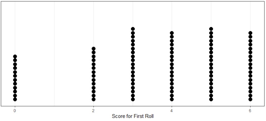
In particular, for the first roll, the possible outcomes of 0,2,3,4,5, or 6 points are equally likely. So the expected score after the first roll is the average of these numbers, \(\frac{20}{6}\), even though there is actually no way to get that score. If we run a simulation with 100 rolls for this situation, we see that each of the outcomes have approximately the same probability of occurring.
If we are in the situation where we have already rolled the die and have points, if we choose to roll during a turn we could expect to earn the average of the possible points on the roll, since all of the possibilities have equal probability. So the expectation is that by rolling again we would have the score of \[\frac{0+(P_0 + 2) + (P_0 + 3) + (P_0+4) + (P_0+5) + (P_0+6) }{6}\] \[= \frac{5P_0 + 20}{6}\]
Related Content Standards
- (HSS.MD.2) Calculate the expected value of a random variable; interpret it as the mean of the probability distribution.
If we consider the sample space, \(\Omega_t\), of a player’s turn in the game of Pig the number of elements in the sample space is much larger. We can also define a function \(X_t:\Omega_t \rightarrow \mathbb{R}\) where \(X_t(\omega)\) is the amount of points corresponding with that sequence of dice rolls for a turn. We will say that \(\verb|turn_points| = X_t(\omega)\).
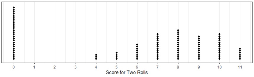
Suppose that we let \(A\subset \Omega_t\) be the possible rolls if we limit a turn to a maximum of two rolls. We have the following possible outcomes for for \(\omega \in A\) with a dot plot of 100 simulations that further shows the distribution of possible scores.
Related Content Standards
- (HSS.MD.1) Define a random variable for a quantity of interest by assigning a numerical value to each event in a sample space; graph the corresponding probability distribution using the same graphical displays as for data distributions.
From this sample of 100 simulations, we see that the average value of the random variable is \(5.95\). Using a sample of 1000 simulations, we find that the average value of the random variable of the score after two rolls is \(5.421\). If we look at all of the possible pairs of rolls for two dice we can determine the probability of getting each possible score value. Since there are 36 different possible rolls for the two dice, we have the following probability distribution.
Probability value of turn_points |
0 | 4 | 5 | 6 | 7 | 8 | 9 | 10 | 11 | 12 |
| Probability of that score in \(A\) | \(\frac{12}{36}\) | \(\frac{1}{36}\) | \(\frac{2}{36}\) | \(\frac{3}{36}\) | \(\frac{4}{36}\) | \(\frac{5}{36}\) | \(\frac{4}{36}\) | \(\frac{3}{36}\) | \(\frac{2}{36}\) | \(\frac{1}{36}\) |
We can then determine the expected value for turn_points with the assumption that there are two rolls by taking a weighted mean.
\[\mbox{Expected Value of a Random Variable}\] \[= \sum (\mbox{possible value}) \cdot (\mbox{probability of that value})\] \[\begin{align} E(X) &= 0 \cdot \frac{12}{36} + 4 \cdot \frac{1}{36} + 5 \cdot \frac{2}{36} + 6 \cdot \frac{3}{36} + 7 \cdot \frac{4}{36} + 8 \cdot \frac{5}{36} \\ & + 9 \cdot \frac{4}{36} + 10 \cdot \frac{3}{36} + 11 \cdot \frac{2}{36} + 12 \cdot \frac{1}{36} \\ &= \frac{4+10+18+28+40+36+30+22+12}{36} \\ &= \frac{200}{36} \\ &= 5 + \frac{5}{9} \end{align}\]
Related Content Standards
- (HSS.MD.3) Develop a probability distribution for a random variable defined for a sample space in which theoretical probabilities can be calculated; find the expected value.
We can also use this terminology to rewrite the expression for the expected value of a discrete random variable \(X\), \[E(X) = \sum_{x} x\cdot P(X=x).\] If \(X\) is a continuous random variable with a probability density function, \(f(x)\), the summation becomes an integral and \[E(X) = \int_{-\infty}^\infty x \cdot f(x) dx.\]
Related Content Standards
(HSS.MD.5) Weigh the possible outcomes of a decision by assigning probabilities to payoff values and finding expected values.
- Find the expected payoff for a game of chance.
- Evaluate and compare strategies on the basis of expected values.
Returning to our game of Pig, recall that the expected value of the score on a turn when rolling the die one time is \(3.667\) and is \(5.556\) when rolling two times. So it seems that the expected value of the score increases as we increase the number of times that we roll the dice on each turn. However, if we think about rolling the dice 20 times on a turn we are almost certain that at least one of those 20 rolls will include a 1 making the expected turn score to be close to 0. This implies that there must be some number of rolls on each turn that would maximize the expected score for a turn. Because the theoretical probabilities become more complicated as we increase the number of rolls on a turn, we can obtain a good estimate for the expected score using 1000 simulations for each number of turns.
From these simulations, we can see that the best strategy, in terms of the number of rolls each turn, is to roll around 5 or 6 times each turn. We could improve our estimates for the expected value by increasing the number of simulations.
| Rolls per Turn | Expected Value | |
|---|---|---|
| 0 | 0.000 | |
| 1 | 3.667 | |
| 2 | 5.421 | |
| 3 | 7.119 | |
| 4 | 7.183 | |
| 5 | 8.060 | |
| 6 | 7.849 | |
| 7 | 7.134 | |
| 8 | 7.283 | |
| 9 | 6.801 | |
| 10 | 5.991 | |
| 11 | 6.157 | |
| 12 | 5.258 | |
| 13 | 4.414 | |
| 14 | 4.327 |
Another option is to run the simulations many times to get a better understanding of the expected values for a turn when rolling 4, 5, 6, 7, or 8 times for a turn. We report the results of 100 experiments of 1000 simulations for each of the options. The mean of the scores for the experiments is equivalent to a mean of a simulation of 100,000 trials.
| Rolls per Turn | Four | Five | Six | Seven | Eight |
| Mean Score | 7.6978 | 8.0453 | 8.0562 | 7.8233 | 7.4375 |
However, we can see from the distributions of these experiments in the box plots below that the expected scores of the 1,000 simulations had some variability.
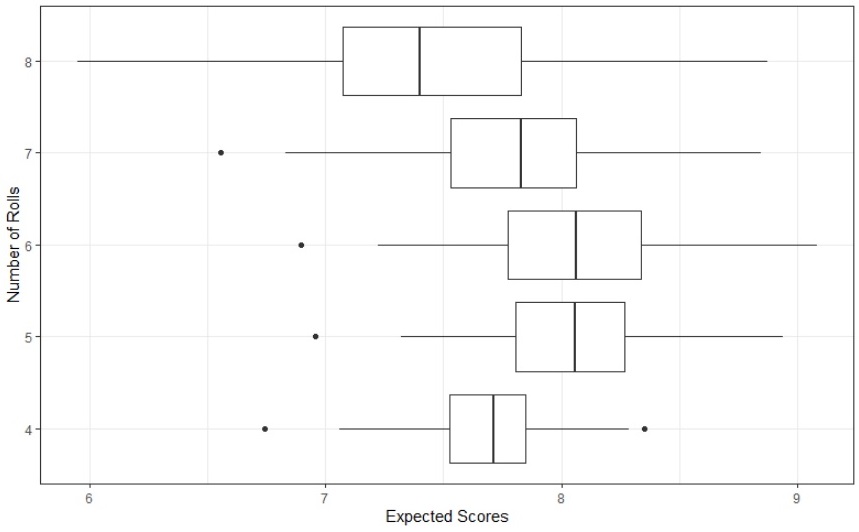
This means that we cannot definitively say if five or six rolls per turn is the best strategy in terms of the number of rolls per turn.
16.4.1 Exercises
Find the best strategy for Pig based on stopping your turn once you have reached a certain number of points for that turn.
Use the theoretical probabilities, Boolean algebra, and conditional probability to determine the expected values for five and six rolls per turn.
In the game of Risk, two players have battles by rolling different numbers of dice. For a battle, the attacker can roll up to 3 dice and the defender can roll up to two dice. Use simulations to analyze the expected value of the number of armies won or lost by the attacker and the defender based on the number of dice chosen by each person for the battle.