17.2 Point and Interval Estimators
Related Content Standards
- (HSS.IC.4) Use data from a sample survey to estimate a population mean or proportion; develop a margin of error through the use of simulation models for random sampling.
Suppose that we want to use the Census at School database to study the properties of secondary school students in the United States. While the sampling of the Census at School website is a sample of convenience, it is unlikely to be biased in the variable of height, but may be biased for other variables as this sample population is more likely to come from schools with higher socioeconomic levels.
Using a sample size of 1000 twelve-year-old students, we find that the sample mean of the heights is 155.485 cm. This is used to estimate the population mean of the heights of twelve-year-old students in the United States. If we had used a different random sample of twelve-year-old students, it is very possible that we would have had a different sample mean. So we would like to get an idea of how well 155.485 cm estimates the actual population mean that would be impossible to compute.
One way to measure how close the sample mean approximates the population mean is to use a simulation. We can randomly select 1000 data points from our sample data using replacements and take the mean of this data set. We can then do this 1000 times to create a distribution of possible means of the heights of twelve-year-old students. We include a sample of code for doing such a simulation in R.
nsims <- 1000 # number of simulations
m <- rep(NA,nsims) # empty vector to store means
for (i in 1:nsims){ m[i] <- mean(sample(Student_twelve$Height_cm, replace = TRUE))}
The result of this loop is a vector with 1000 means of the simulated sample heights.
We find that the mean of the simulations is also 155.47 cm and has a standard deviation of 0.364 0.365 cm. We also have the 95% of the simulations fell between 154.759 and 156.192. So we call the interval (154.759,156.192) a 95% confidence interval (95% CI) for the mean of the heights of the population. While this does not assure that the actual population mean is inside of this interval, we can be fairly certain that our interval contains the population mean.
We can notice that the density curve of the average heights of 1000 samples appears to be a normal distribution. If we look at similar density curves for average heights of 20, 100, and 500 samples we see that the shape of the curve is seeming to approach a normal distribution.
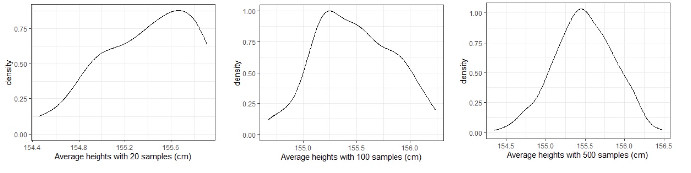
This property that the distribution of the averages of \(n\) samples approaches a normal distribution is the Central Limit Theorem.
Theorem 17.1 (Central Limit Theorem) If \(S_n\) is the sum of \(n\) mutually independent random variables, then the distribution function of \(S_n\) will approach a normal distribution as \(n\rightarrow \infty\).
So, if our random variable of interest for the entire population, \(X\), has a mean \(\mu\) and standard deviation \(\sigma\), the Central Limit Theorem implies that \[\mu = E(\overline{X}) \quad \mbox{ and } \quad \sigma_{\overline{X}}= \frac{\sigma}{\sqrt{n}}.\]
17.2.1 Estimating Population Means and Medians
Using the Central Limit Theorem, we can compute the standard error for the sample mean of the heights, \[ \sigma_{\overline{Y}} = \frac{\sigma}{\sqrt{n}} \approx \frac{11.52035}{\sqrt{1000}} \approx 0.364 \mbox{cm}.\] We can also create a 95% confidence interval using the knowledge the 95% of the data in a normal distribution falls between \(1.96\) standard deviations below the mean and \(1.96\) standard deviations above the mean so that we have \[( \overline{X} - 1.96 \sigma_{\overline{X}}, \overline{X} + 1.96 \sigma_{\overline{X}}) = (154.772, 156.198) .\]
Notice that the standard deviation of the means of the heights corresponds to the algebraic standard error expression. In this case, the algebraic expression is much more efficient than the simulation. However, there are cases in which a simulation is more effective. For instance, if we want to find the standard error of the median of a random variable that does not have a normal distribution, the algebraic methods would not work and we would need to use a simulation.
Consider the number of texts received by twelve-year-old students. We can see in the density plot below, this variable does not follow a normal distribution and the center of the data is best represented by the median.
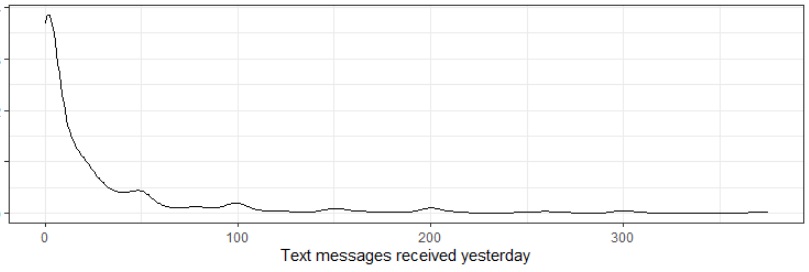
We see that the median number of text messages received yesterday from our sample of 1000 twelve-year-old students was 7 messages. Using 1000 simulations we see that the average of these medians was 7.219 text messages with a standard error of 1.015 messages. Using the simulation technique for estimating a 95% confidence interval generates an interval of (6,10), while the Central Limit Theorem method of estimating a 95% confidence interval generates an interval of (5.230, 9.208). Since the median of the population is likely to be a natural number, the interval of (6,10) is probably more appropriate for this setting.
17.2.2 Estimating Differences of Means
If we want to compare the heights of twelve-year-old students and seventeen-year-old students, we can use the Census at School random sampler to generate a random sample of seventeen-year-old students from the United States. The average height of students in this sample is 171.105 cm. This seems to be significantly different from the average height of the twelve-year-old students, 155.485 cm, but it would be useful to have a way to test for such a difference. A standard process to determine if there is a difference between two means is to consider the random variable of the differences between the means of the samples, \((\overline{X_1} - \overline{X_2})\), which estimates the differences in the means of the populations, \((\mu_1-\mu_2)\). The Central Limit Theorem implies that the standard error for this point estimator is \(\displaystyle{\sqrt{ \frac{\sigma_1^2}{n_1} + \frac{\sigma_2^2}{n_2}}}\).
Since the standard deviation of the height of the sample of twelve-year-old students is 11.520 and the standard deviation of the height of the sample of seventeen-year-old students is 12.489, we see that the standard error for the difference of means is \[\sigma_{(\overline{X_1}-\overline{X_2})} = \sqrt{\frac{12.489^2}{1000} + \frac{11.520^2}{1000} } = 0.537\] and so the 95% confidence interval for the difference in means is \((14.57, 16.67)\). If the means of the two populations are the same, then the expected value of the difference in means would be zero. Since zero is not inside of this confidence interval, we can infer that the difference in heights is significant.
If we look at a sample of 1000 thirteen-year-old students we see that the average height of the 510 Females is 160.1176 and the average height of the 488 Males is 162.707. Using the standard deviations of the two samples we see that the standard error for the difference in means is \[\sigma_{(\overline{X_1}-\overline{X_2})} = \sqrt{\frac{12.88^2}{488} + \frac{9.71^2}{510} } = 0.72\] producing a 95% confidence interval for the difference between the means of (1.17, 4.01). A similar process for the 1000 twelve-year-old students estimates the average height of twelve-year-old females as 155.4825 (\(n_1=485\)) and males as 155.4874 (\(n_2=515\)) with a confidence interval for the difference in means of (-1.42, 1.43). So we can infer that there is no significant difference in the average heights of twelve-year-old students, but there is a significant difference in the average heights of thirteen-year-old students, based on gender.
Related Content Standards
- (HSS.IC.4) Use data from a sample survey to estimate a population mean or proportion; develop a margin of error through the use of simulation models for random sampling.
17.2.3 Estimating Proportions
There are many times that we would like to find the proportion of the population that satisfies a certain condition. Election polling estimates the proportion of the population that will vote for certain candidates in an upcoming election. There are many times where a study wants to know the percentage of the population with certain demographic characteristics such as gender, race, or age.
If the proportion of the population that satisfies a certain condition is given by \(p\), then in a random sample of size \(n\) we can label the outcome of the trial for each sample as \(Y_i\) whose value is a 0 if it does not satisfy the condition or a 1 if it satisfies the condition. So the expected value of the sample would be \[E(X) = E\left(\sum_{i=1}^n Y_i\right) = \sum_{i=1}^n E(Y_i) = \sum_{i=1}^n 1\cdot p = np\] since each of the cases is independent of the other cases. Therefore, we can estimate the proportion of the population with the proportion of the sample, \(\hat{p} = \frac{X}{n}\).
Since the variance of a random variable, \(X\), is the expected value of the squared deviation from the mean of \(X\), \(E(X)\), \[\mbox{Var}(X) = E\left( (X-E(X))^2\right),\] we can rewrite this expression as \[\begin{align} \mbox{Var}(X) &= E\left( (X-E(X))^2\right) = E\left( X^2-2XE(X) + E(X)^2\right) \\ &= E(X^2)-2E(X)E(X)+E(X)^2 = E(X^2)-E(X)^2. \end{align}\] So \[\mbox{Var}(X) = E(X^2)-E(X)^2 = E(X(X-1))+E(X)-E(X)^2 = n(n-1)p^2 + np - (np)^2 = np(1-p)\] and the standard error of our estimator is \[\sigma_{\hat{p}} = \sqrt{\frac{p(1-p)}{n}}.\]
These estimators are appropriate once the binomial distribution approaches a normal distribution, with often occurs once both \(np\) and \(n(p-1)\) are greater than 5.
From September 30 to October 3, 2020, Auburn University at Montgomery surveyed 1,072 registered voters and found that 397 people planned to vote for Biden and 611 people planned to vote for Trump in the 2020 Presidential election. We can then use simulations to create a confidence interval estimate for the percentage of the vote in Alabama that Donald Trump would earn.
cand = c(1,0)
px = c(0.57, 0.43)
nsims <- 1000 # number of simulations
m <- rep(NA,nsims) # empty vector to store means
for (i in 1:nsims){ m[i] <- mean(sample(cand, size=1072, replace=TRUE, prob=px))}
quantile(m,c(0.025,0.975))
This gives us a 95% confidence interval of \((0.54,0.60)\) for the percentage of votes for Donald Trump in Alabama in 2020. This matches exactly the 95% confidence interval found using the standard error for the estimate, \[\left( 0.57-1.96 \cdot \sqrt{\frac{(0.57)(1-0.57)}{1072}}, 0.57+1.96 \cdot \sqrt{\frac{(0.57)(1-0.57)}{1072}}\right) = (0.54,0.60).\]
17.2.4 Interpretations
The best way to understand a 95% confidence interval is that if one repeated the sampling procedure 100 times and created 100 95% confidence intervals, one would expect that 95 of these would contain the actual value of the parameter being estimated. So if we are comparing an estimate of a parameter for two samples and the 95% confidence intervals of these samples do not overlap we can be fairly confident the the values of the population parameters being estimated are distinct. If the confidence intervals overlap, we need to use other pieces of evidence to build an argument for the existence or non-existence of a difference between the two populations.
17.2.5 Exercises
In a study to measure the effects of texting while driving (He et al., 2014), 35 college-age participants were tested on their brake response times under different conditions in a driving simulator. For the drive-only condition, the brake response times had a mean of 1.49 s with a standard deviation of 0.56 s. This leads to a 95% confidence interval of \((1.30,1.68)\). A condition of driving while using a verbal texting system had a mean of 1.63 s with a standard deviation of 0.47 s, giving a 95% confidence interval of \((1.47,1.79)\). The condition of driving and manually texting had a mean of 1.73, standard deviation of 0.48 s with a 95% confidence interval of \((1.57, 1.89)\).
- What conclusions can be drawn from these results and how would you provide evidence for your assertions?
- If you wanted to replicate this study with a stronger set of evidence, what sample size would be required? Explain your reasoning.