16.2 Probability Spaces

Throughout this section we will define many different terms and develop a great deal of notation regarding the theory of probability. In order to assist us in this process we will use the game of Pig as a concrete example to study.

There are many different variations of the game of Pig, but the one that we will begin with involves the rolling of a single die. For each turn, a player repeatedly rolls a die until either a \(1\) is rolled or the player decides to ‘hold’. If the \(1\) is rolled, the player scores nothing on that turn and it becomes the next player’s turn. If a \(1\) is not rolled, the player chooses to either roll again or ‘hold’. If the player chooses to ‘hold’, that player receives a score for that turn of the sum of the rolls up to that point. This score on the turn is then added to the player’s previous score to create the total score. The players then take turns until one player has a total score of 100 points.

In order to better understand this process we will create an example game.

• Player 1: Rolls a 3 and decides to roll again and rolls a 1. This player gets no points for the turn.
• Player 2: Rolls a 4, then a 5, then a 2 and decides to hold. This player gets 11 points for the turn.
• Player 1: Rolls a 6 and a 2 and decides to hold with 8 points for the turn.
• Player 2: Rolls a 3 and a 2 and decides to hold. Player 2 now has 5 points for the turn and 16 total points.
• Player 1: Rolls a 1. Player 1 gets 0 points for the turn and has 8 total points.
• Player 2: …

So for each roll, a player has six possible outcomes on the die, \(\{1,2,3,4,5,6\}\). This set of possible outcomes is called the sample space of the random phenomenon of rolling a die.

Definition 16.1 The sample space, \(\Omega\), is the set of all possible outcomes of a random phenomenon. An outcome, \(\omega\), is an element of the sample space (\(\omega \in \Omega\)).

An event \(A\) is a subset of the sample space, \(A \subseteq \Omega\). If the random phenomenon give the outcome \(\omega\), we say that event \(A\) occurred if \(\omega \in A\).

In the game of Pig we can consider the set of possible rolls in a turn to be the sample space under consideration. In this situation, each outcome, or element of the sample space, would be a sequence of rolls of the die, with all but a finite number being blank. So one possible outcome would be \[\omega = (2,3,6,5,1,.,.,\ldots)\] if a person rolled a 2, then a 3, then a 6, then a 5, then a 1. After the roll of the 1, there would not be any more rolls. An event would be a set of outcomes, or turns.

Now that we have the idea of a sample space we are ready to define the probability for events in that sample space.

Definition 16.2 Let \(\Omega\) be a sample space of outcomes and let \(\mathcal{F}\) be a collection of subsets of \(\Omega\) that satisfy the following (\(\sigma\)-field) properties:

• (S1) \(\Omega \in \mathcal{F}\)
• (S2) If \(A\in \mathcal{F}\), then \(A^c = \Omega\setminus A \in \mathcal{F}\).
• (S3) If \(I\) is a finite or countably infinite indexing set and \(\left\{A_i \right\}_{i\in I} \subset \mathcal{F}\), then \(\bigcup_{i\in I} A_i \in \mathcal{F}\).

A function \(P:\mathcal{F} \rightarrow [0,1]\) is called a probability measure if it satisfies the following properties:

• (P1) \(P(\Omega) = 1\) and \(P(\emptyset)=0\)
• (P2) For all events \(A \in \mathcal{F}\), \(0\leq P(A) \leq 1\).
• (P3) If events \(A_1, A_2, \ldots \in \mathcal{F}\) are mutually disjoint (\(A_i \cap A_j = \emptyset\) for all \(i\neq j\)), then \[P\left(\bigcup_{i=1}^\infty A_i \right) = \sum_{i=1}^\infty P(A_i)\]

The \(\sigma\)-field properties of \(\mathcal{F}\) ensure that the corresponding properties of \(P\) make sense. Most of the sample spaces encountered in the K-12 curriculum are finite spaces and the collection of subsets, \(\mathcal{F}\), of \(\Omega\) is usually just the power set of \(\Omega\).

If \(\Omega\) is a non-empty set, we know that \(\Omega \in \mathcal{F}\) and property (S2) says that \(\emptyset\in \mathcal{F}\). So the smallest collection of subsets of \(\Omega\) that satisfy these conditions is \(\left\{ \emptyset, \Omega \right\}\).

Using the generalized De Morgan’s Laws (Theorem 2.7), \[\bigcap_{i\in I} A_i = \left( \bigcup A_i^c \right)^c\] we can combine properties (S2) and (S3) to see that the intersections of sets in \(\mathcal{F}\) is also in \(\mathcal{F}\).

The requirement that \(P(\Omega)=1\) ensures that the probability of all possible outcomes is 1. Similarly, \(P(\emptyset)=0\) is that the option of no outcome occurring is not possible.

The requirement that \[P\left(\bigcup_{i=1}^\infty A_i \right) = \sum_{i=1}^\infty P(A_i)\] when the \(A_i\) are mutually disjoint is often referred to as the countable additivity of the probability measure. Another way of describing mutually disjoint events is mutually exclusive.

Definition 16.3 Two events are mutually exclusive events if they cannot happen at the same time. \[A\cap B =\emptyset\]

In our example of playing Pig with only rolling two times on each turn we can rewrite some of our information using this new terminology. We can consider \(\Omega\) to be the possible pairs of rolls, \[\Omega = \left\{ (a,b) \vert a,b\in \{1,2,3,4,5,6\} \right\}\] and \(\mathcal{F} = \mathcal{P}\left(\Omega \right)\). Then the probability of rolling a \(1\) for at least one of the rolls would be \[P\left( \left\{ (1,1), (1,2), (1,3), (1,4), (1,5), (1,6), (2,1), (3,1), (4,1), (5,1), (6,1) \right\} \right) = \frac{11}{36}\] and so the probability of getting zero points for a turn using the two rolls strategy is \(\frac{11}{36}=30.5\%\).

If we change the strategy to rolling three times on each turn, we see that the probability of rolling a 1 for at least one of the rolls would be \(1-P(\mbox{not rolling a 1})\). And we see that the probability of not rolling a 1 for any of the three rolls would be \[\frac{5}{6}\cdot \frac{5}{6} \cdot \frac{5}{6}= \frac{125}{216}.\] So the probability of rolling at least one 1, would be \(42.1\%\).

So we see that as the number of rolls per turn increases, it is more likely to not score any points on a turn.

16.2.1 Boolean Algebra and Probability

Since \(P\) maps subsets of \(\Omega\) into the interval \([0,1]\) we need to understand how \(P\) operates with Boolean algebra, the algebra of sets, and how that relates to the language of probability.

We first note that for two sets \(A,B\subseteq \Omega\), \(A\cap B\) is the set of outcomes in \(\Omega\) that are in both \(A\) and \(B\). In our example from the game of Pig with rolling twice for a turn, we can let \(A\) be the set of events where a 3 is rolled on the first roll. So \[A = \left\{ (3,1), (3,2), (3,3), (3,4), (3,5), (3,6)\right\} \mbox{ and } P(A) = \frac{6}{36}.\] Let \(B\) be the set of events where a 4 or 5 is rolled on the second roll, \[B=\left\{ (1,4), (2,4), (3,4), (4,4), (5,4), (6,4), (1,5), (2,5), (3,5), (4,5), (5,5), (6,5)\right\} \mbox{ and } P(B) = \frac{12}{36}.\] Then \(A\cap B\) is the set of events where a 3 is rolled on the first roll and a 4 or 5 is rolled on the second roll, \[A\cap B = \left\{ (3,4), (3,5)\right\} \mbox{ and } P(A\cap B) = \frac{2}{36}.\]

Related Content Standards

• (HSS.CP.1) Describe events as subsets of a sample space (the set of outcomes) using characteristics (or categories) of the outcomes, or as unions, intersections, or complements of other events (“or,” “and,” “not”).

Similarly, \(A\cup B\) is the set of events that occur in either \(A\) or \(B\), or both. In our example above, \[A\cup B = \left\{ (3,1), (3,2), (3,3), (3,4), (3,5), (3,6), (1,4), (2,4), (4,4), (5,4), (6,4), (1,5), (2,5), (4,5), (5,5), (6,5)\right\}\] and \(P(A\cup B) = \frac{16}{36}\).

We can notice that \[P(A\cup B) = P(A) + P(B) - P(A\cap B).\]

The following theorem generalizes this result and describes how probability measures interact with Boolean algebra of sets.

Theorem 16.1 If \(A, B\in \mathcal{F}\) and \(P:\mathcal{F}\rightarrow [0,1]\) is a probability measure, then

1. \(P(A^c) = 1- P(A)\)
2. \(P(A \setminus B) = P(A) - P(A\cap B)\)
3. \(P(A \cup B) = P(A)+P(B) - P(A\cap B)\)
4. If \(A\subseteq B\), then \(P(A)\leq P(B)\).

Proof. Proof of (a): Since \(A\in \mathcal{F}\), property (S2) says that \(A^c\) is also in \(\mathcal{F}\) and so \(P(A^c)\) is well-defined. We also know that \(\Omega = A \cup A^c\) and that \(A\cap A^c = \emptyset\). So property (P3) states that \[ P(\Omega) = P(A) + P(A^c).\] Since \(P(\Omega)=1\), we have that \(P(A^c)=1-P(A)\).

Proof of (b): Let \(A,B\in \mathcal{F}\). Since \(\Omega = B \cup B^c\), we know that \[A = A \cap \Omega = A \cap (B \cup B^c) = (A\cap B) \cup (A \cap B^c) = (A\cap B) \cup (A \setminus B).\] Since \((A\cap B)\) and \(A\setminus B\) are disjoint, property (P3) gives us that \(P(A) = P(A\cap B) + P(A \setminus B)\). We can rearrange this equation so that \[P(A\cap B) = P(A) - P(A\setminus B).\]

Proof of (c): Let \(A,B\in \mathcal{F}\). Then we know that \[(A\setminus B) \cup (A\cap B) \cup (B\setminus A)\] is a partition of \(A\cup B\) in that the three sets are mutually disjoint and their union is \(A\cup B\). So \[P(A\cup B) = P(A\setminus B) + P(A\cap B) + P(B\setminus A)\] by property (P3). Combining this with part (b) of the theorem we have \[P(A\cup B) = (P(A)-P(A\cap B)) + P(A\cap B) + (P(B)-P(A\cap B)) = P(A) + P(B) - P(A\cap B).\]

Proof of (d): Let \(A,B\in \mathcal{F}\) such that \(A\subseteq B\). Since \(A\subset B\), \[B= B \cap (A \cup A^c) = (B\cap A) \cup (B\cap A^c) = A \cup (B\setminus A)\] and \(A\) and \(B\setminus A\) are disjoint. So property (P3) gives us that \(P(B) = P(A) + P(B\setminus A)\). Since \(P(B\setminus A) \geq 0\), \(P(A) \leq P(B)\).

Related Content Standards

• (HSS.CP.7) Apply the Addition Rule, \(P(A \mbox{ or } B) = P(A) + P(B) - P(A \mbox{ and } B)\), and interpret the answer in terms of the model.
  

A common example used to better understand the usefulness of the language of probability is called the ‘Monty Hall’ problem as it is based on a scenario from the game show ‘Let’s Make a Deal’ hosted by Monty Hall. In this scenario there are three doors in the game show studio. Behind one of the doors is a new car. Behind the other two doors is a goat. The contestant is asked to choose which door they think the car is behind. Monty then reveals the goat behind one of the doors that was not chosen and asks the contestant if they would like to stick with their current door or change to the new door. Because of the condition and event that one of the doors has been revealed, we see that the probability of a car behind each door has changed.

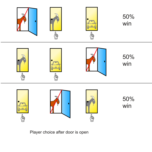
Figure 16.1: Monte Hall Problem

We will denote the sample space in this problem as \[\Omega = \left\{ CGG, GCG, GGC\right\}\] where \(CGG\) denotes that the car is behind Door 1. Assume that a contestant originally chooses Door 2. Since \(P(\{GCG\})=\frac{1}{3}\) their probability of winning the car is \(\frac{1}{3}\). Monty then reveals that the car is not behind Door 3 so that \(P(\{GGC\})=0\). This means that \(P(\{CCG\})=\frac{2}{3}\), meaning that the player should definitely change their choice of doors because it doubles their chance of winning a car.

We can verify this conclusion by assuming that the contestant chooses Door 1 and look at the possible outcomes.

Table 16.5:

	Behind Door 1	Behind Door 2	Behind Door 3	Result if Staying	Result if Switching
	Car	Goat	Goat	Wins Car	Loses
	Goat	Car	Goat	Loses	Wins Car
	Goat	Goat	Car	Loses	Wins Car

16.2.2 Exercises

1. How likely is it that a family with five children has all boys or all girls?

   1. Answer the question by listing out all of the possible combinations of boys and girls.
   2. Show a tree diagram of this scenario.
   3. Answer the question using a simulation and estimating the probability.
   4. Answer the question using properties of compound events.
   5. Compare and contrast the different methods.
   6. How would the different methods perform with changing the question to ‘How likely is it that a family with five children has exactly two girls?’ or ‘How likely is it that a family with five children has at least two girls?’